machine learning, ai, cs · slides

Paper overview | Mastering the game of Go with deep neural networks and tree search
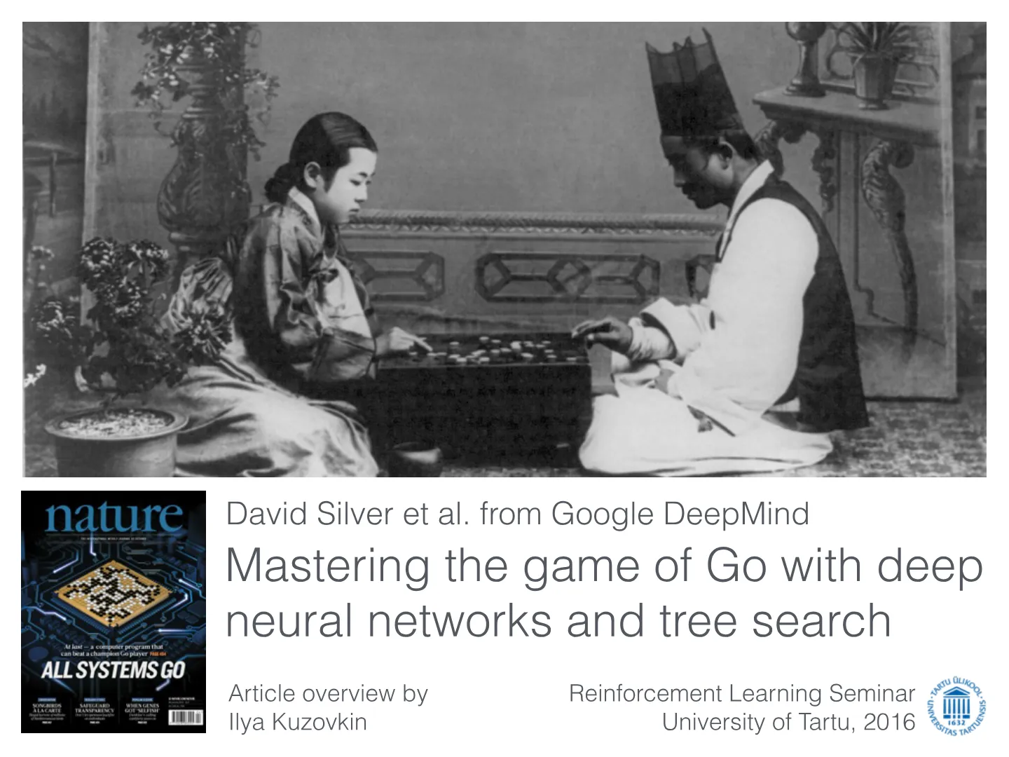
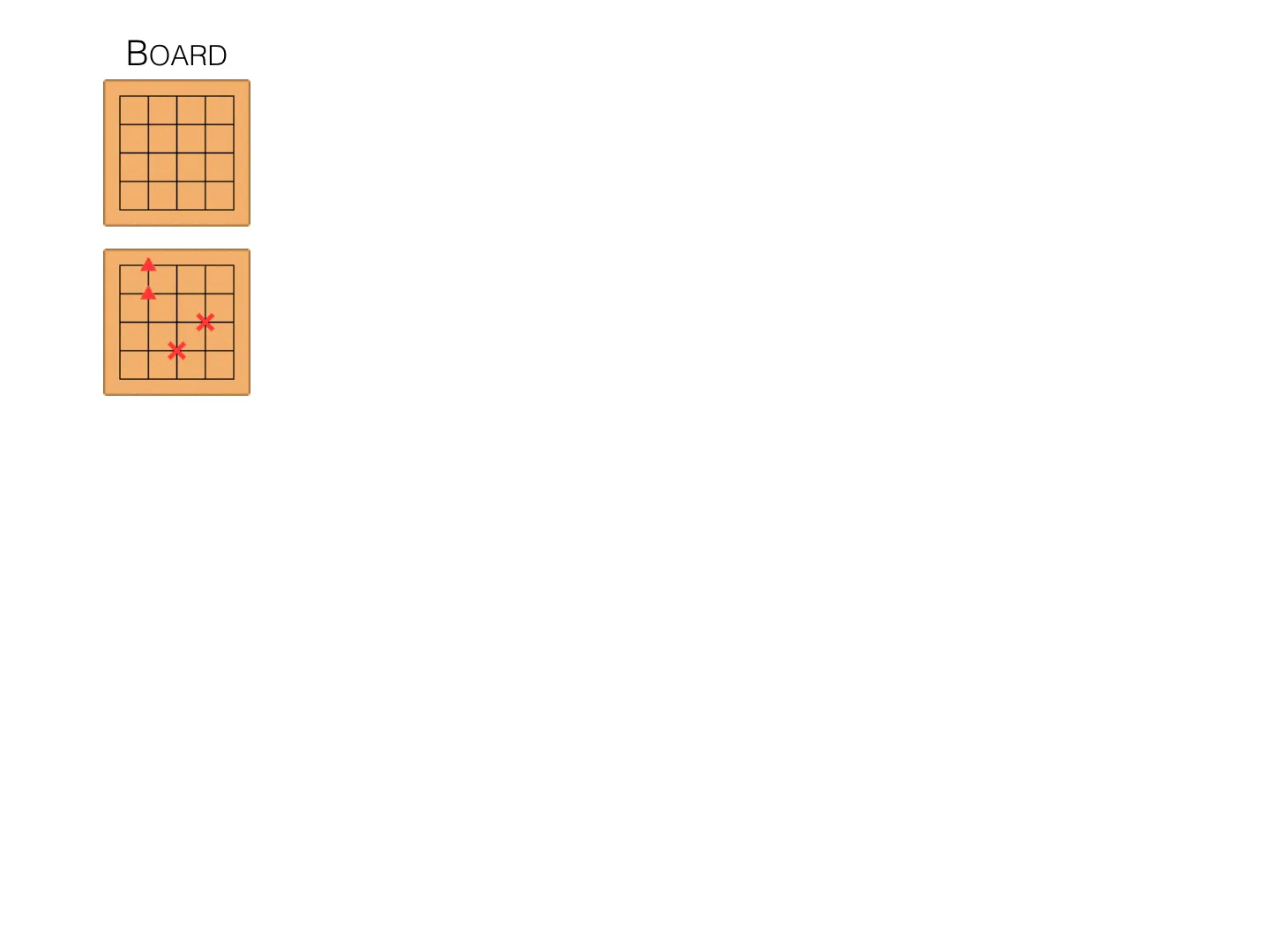
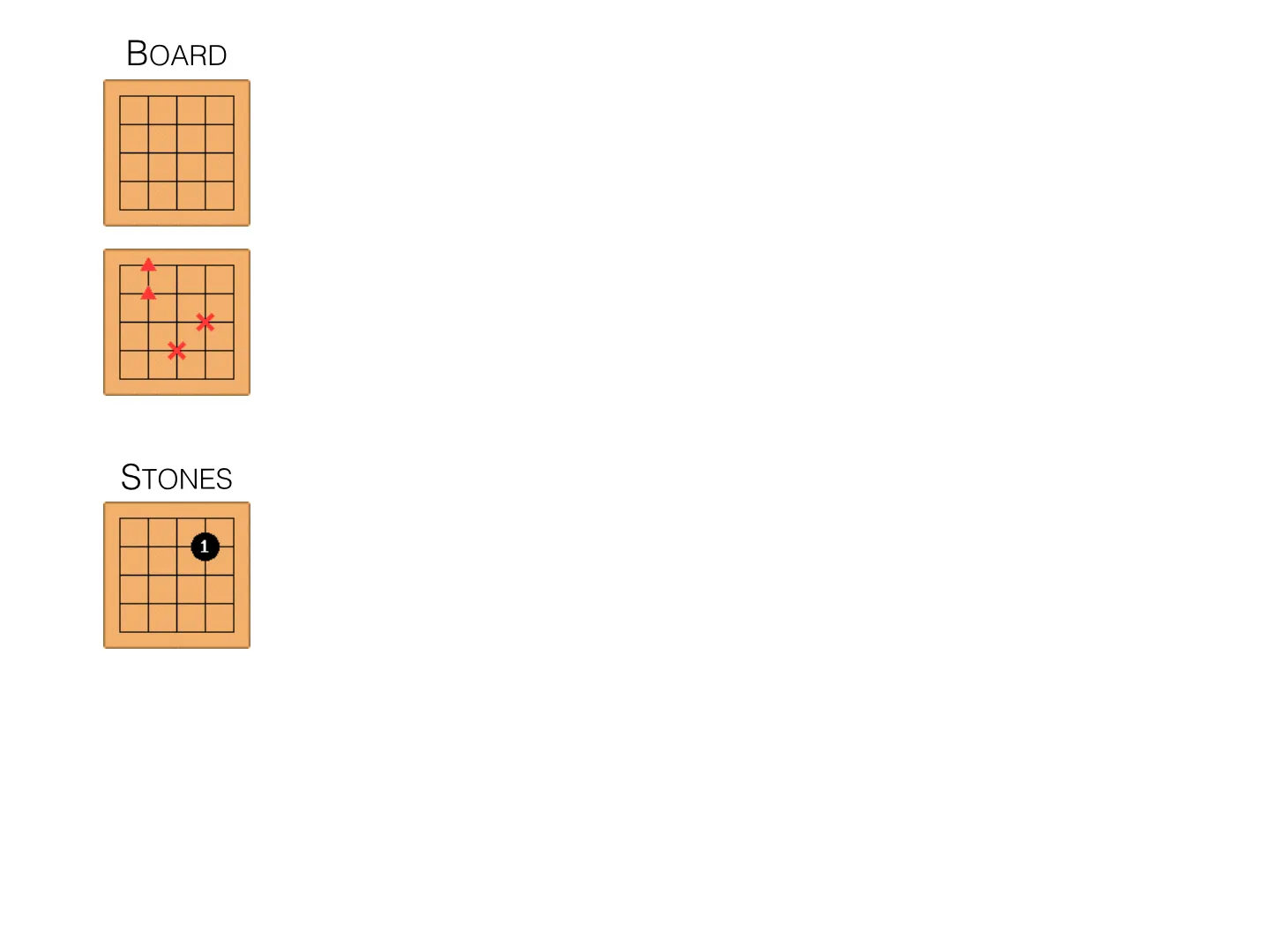
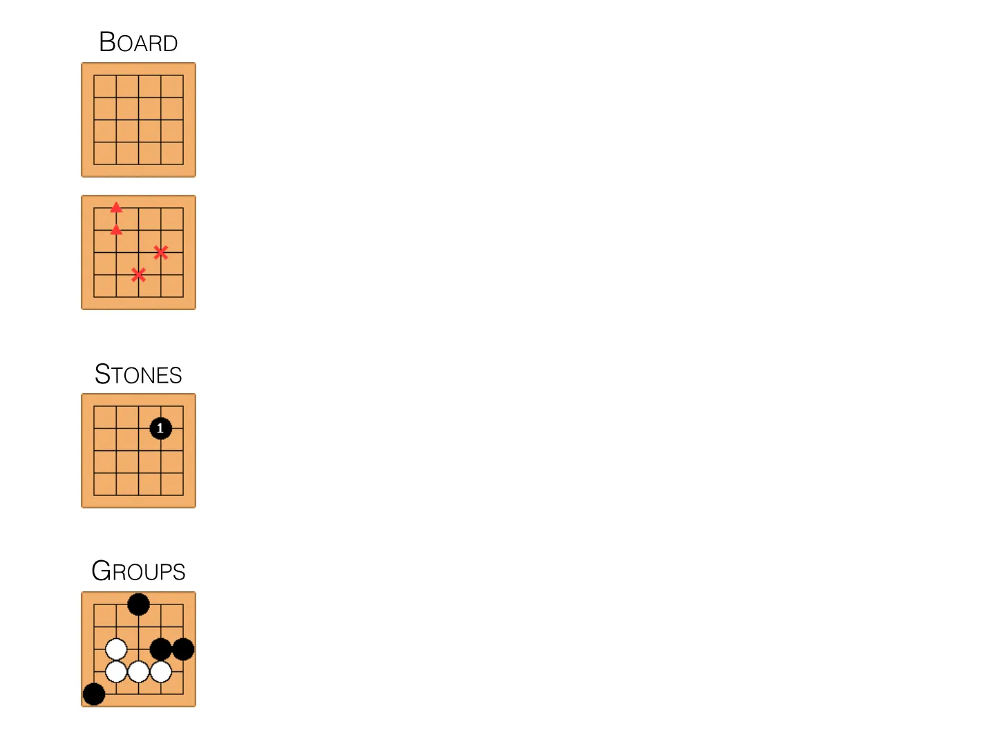
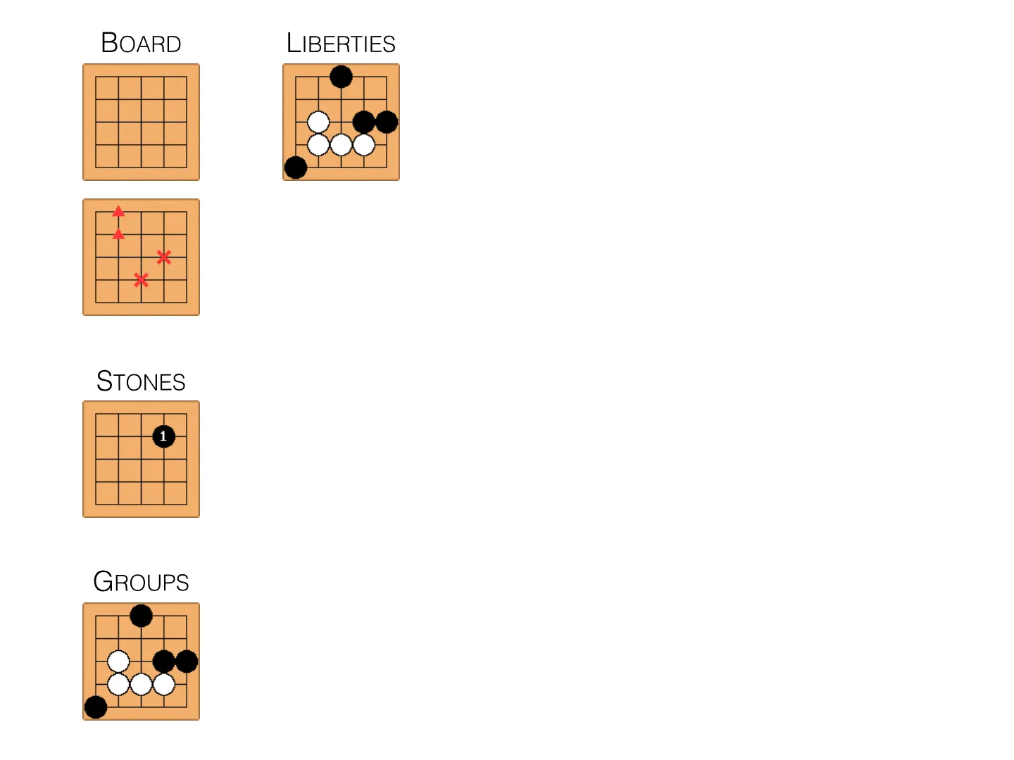
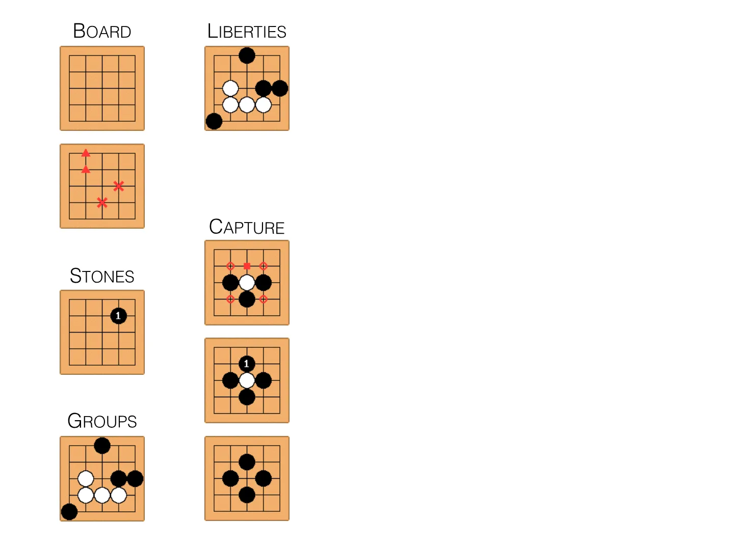
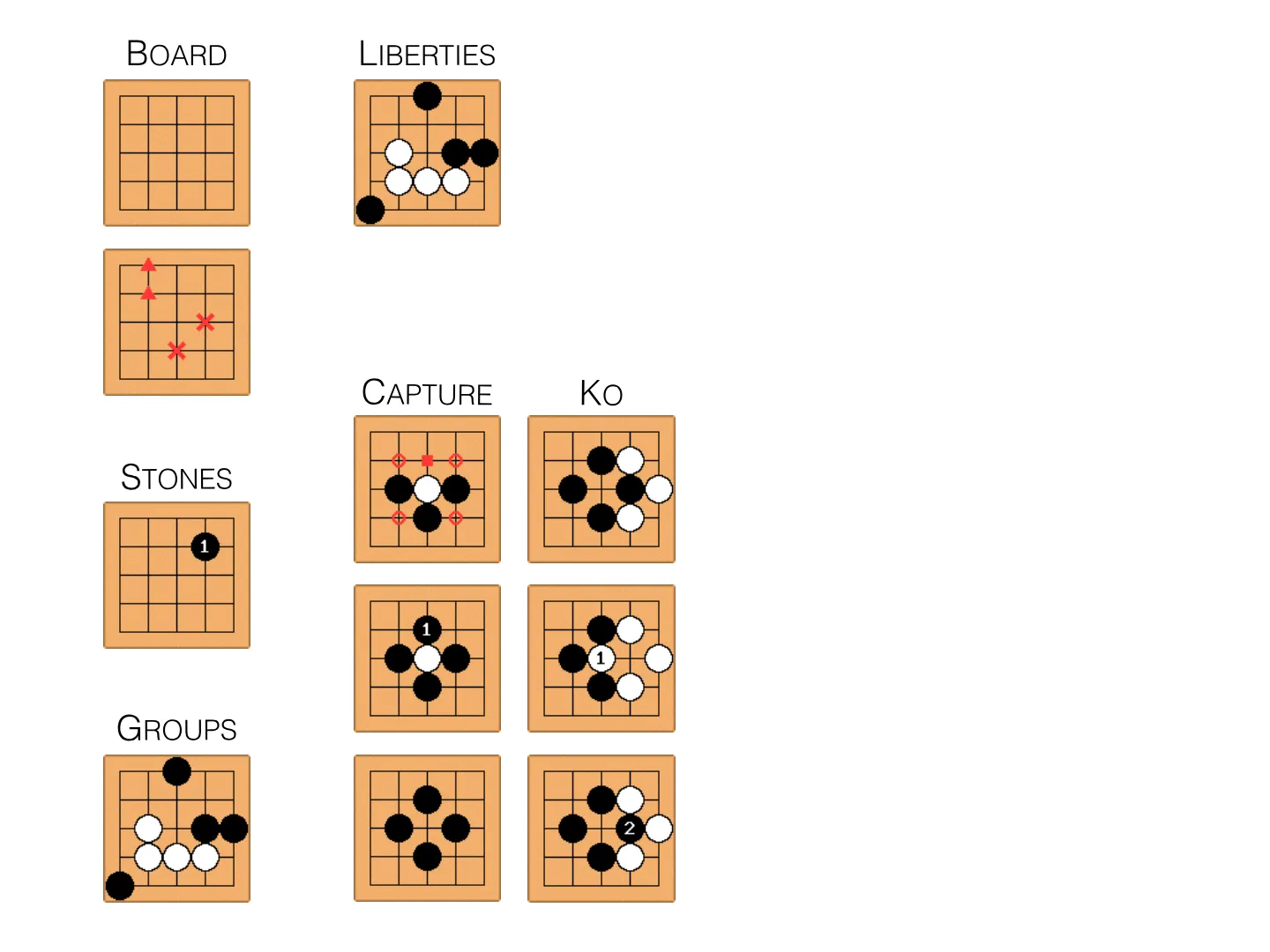
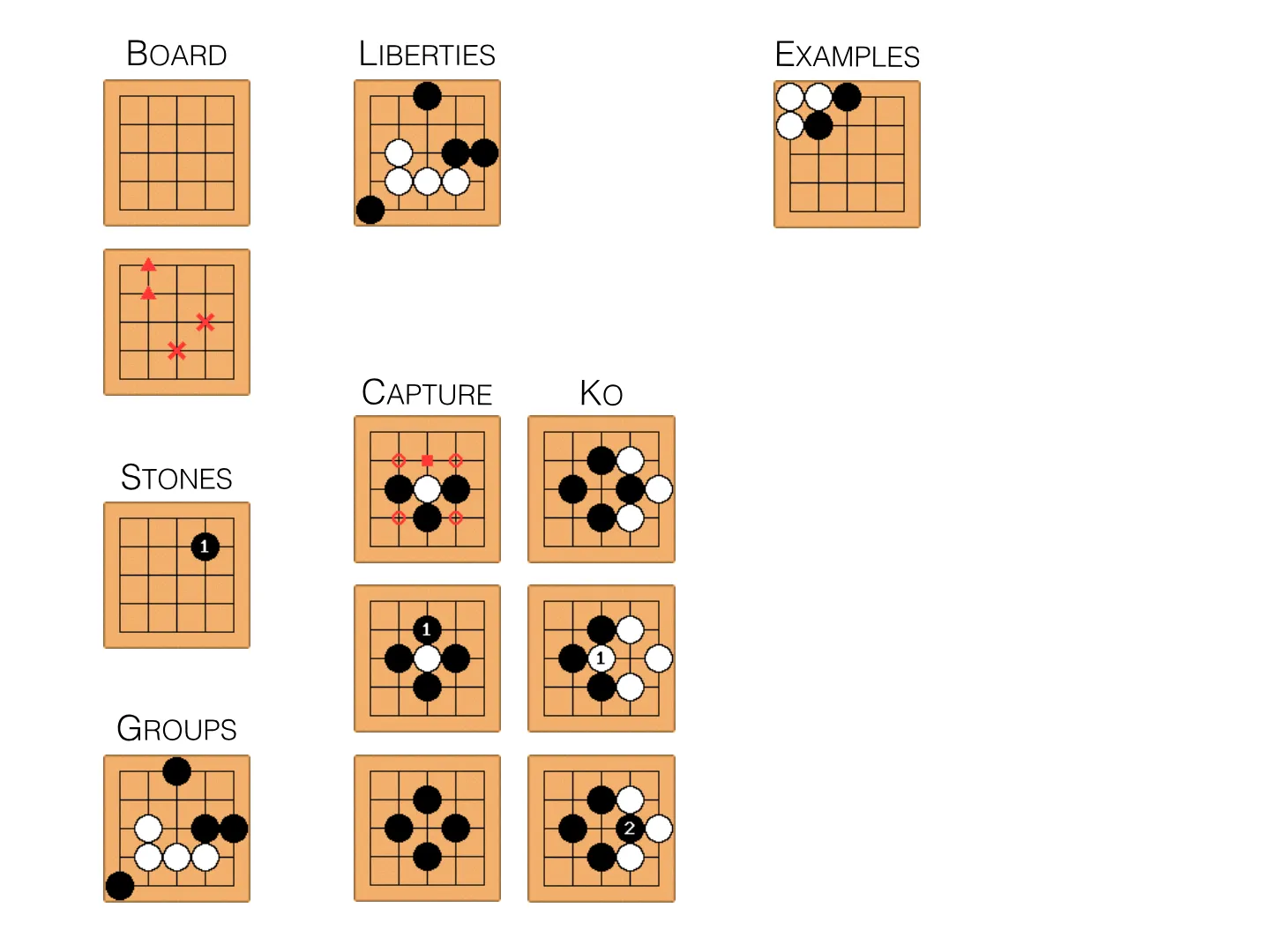
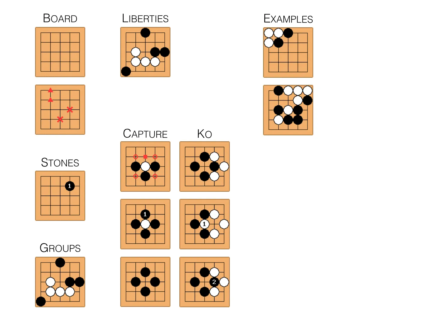
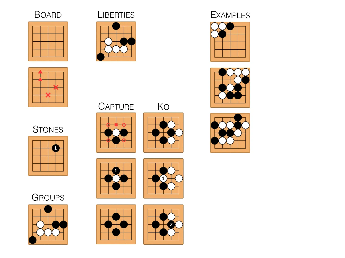
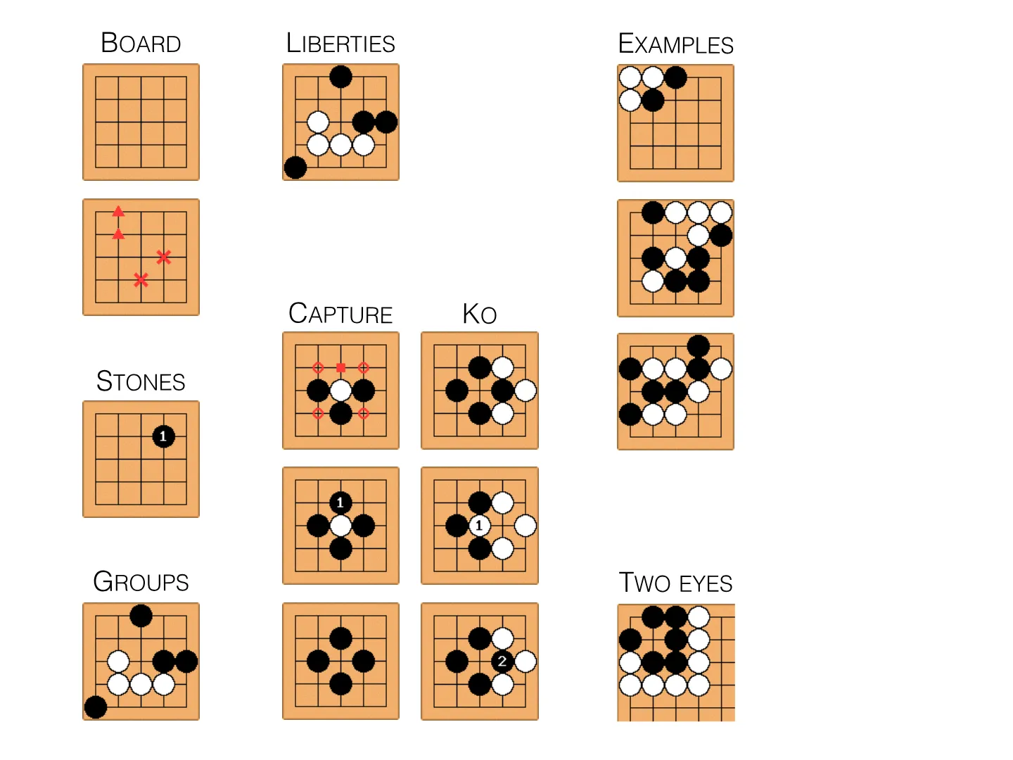
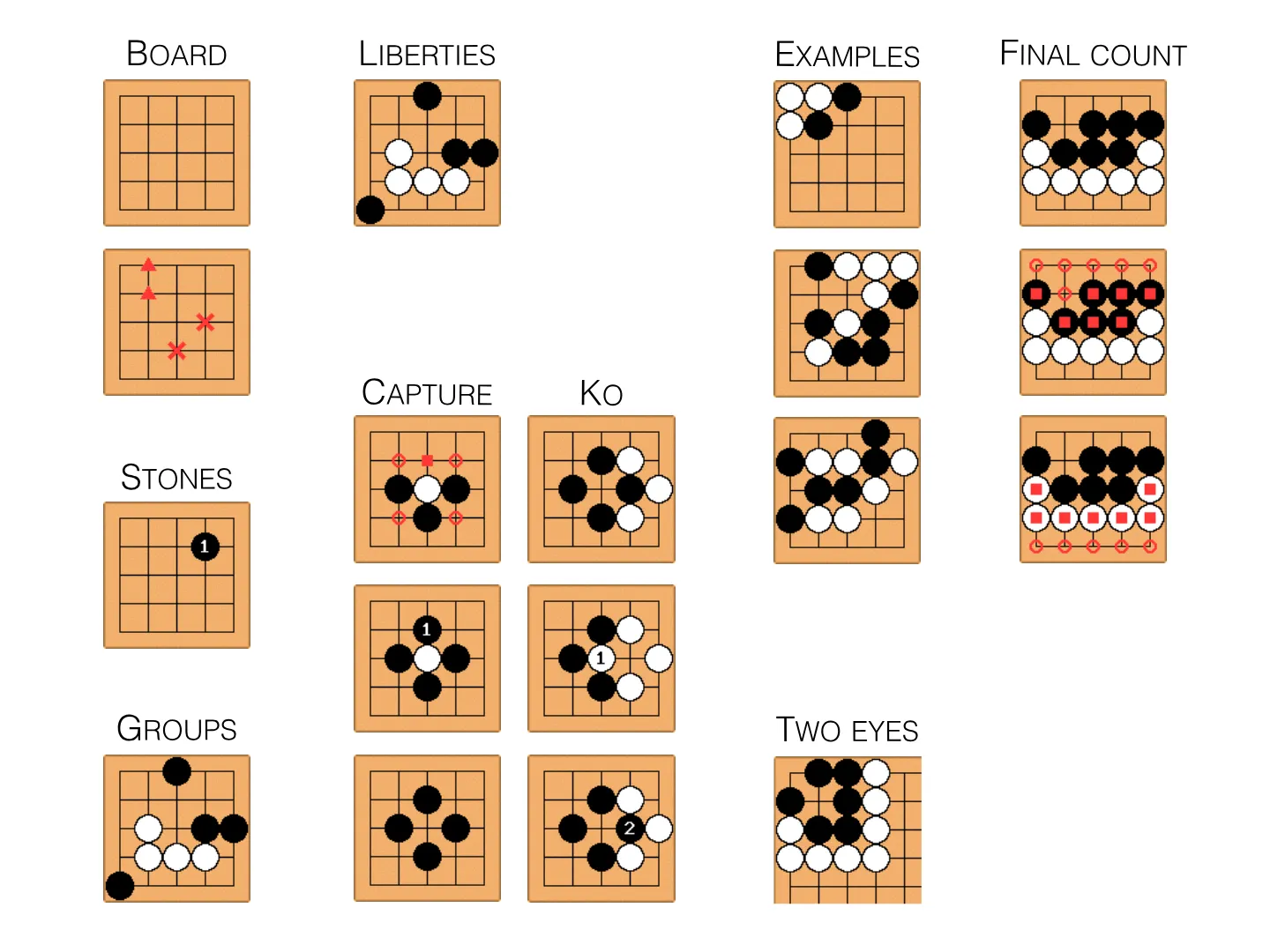
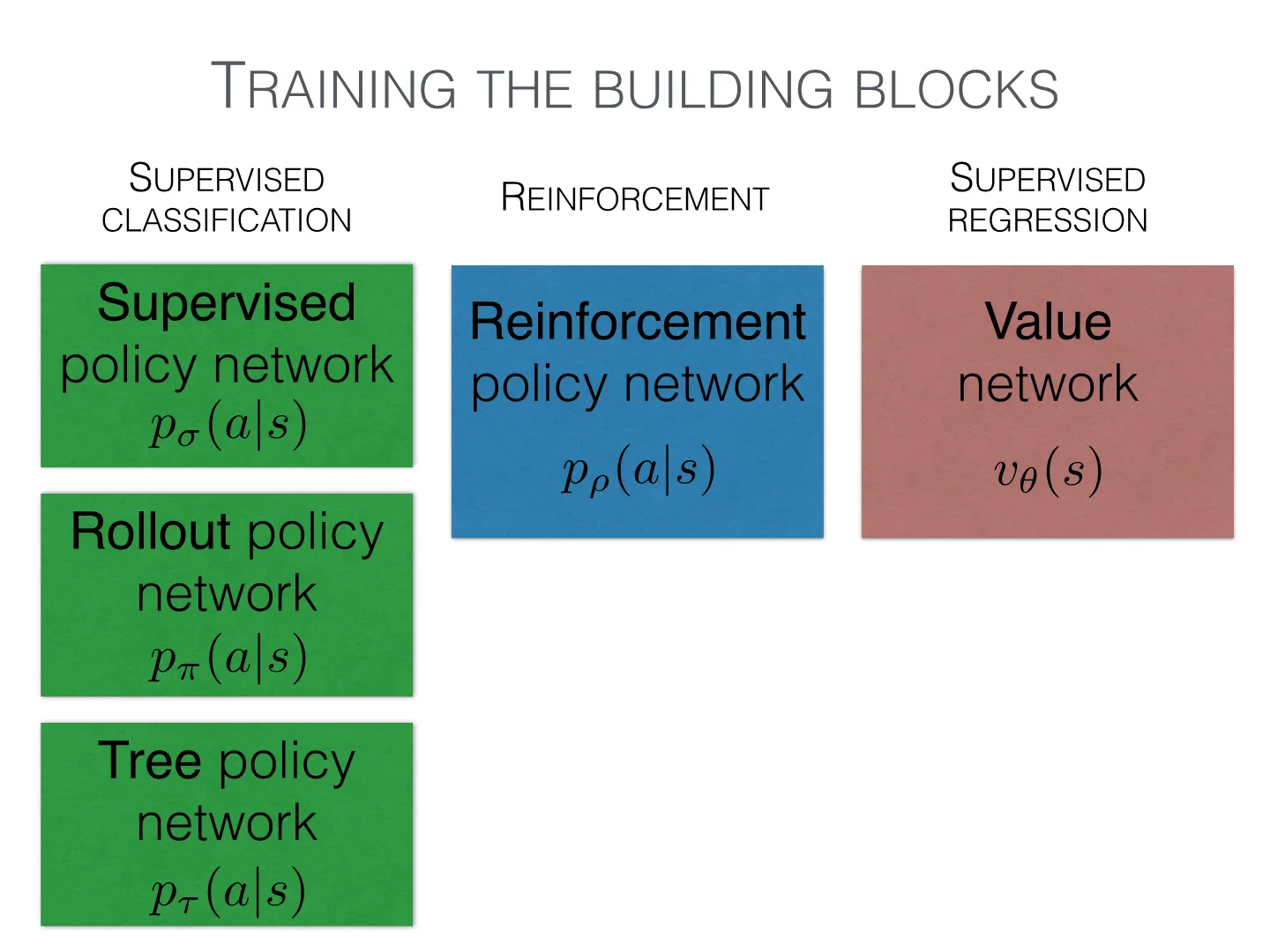
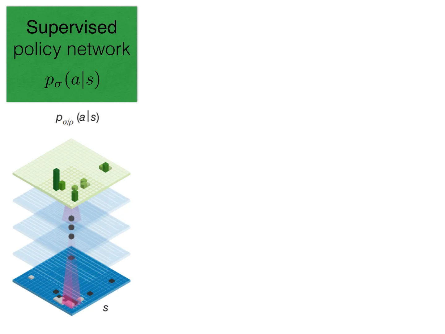
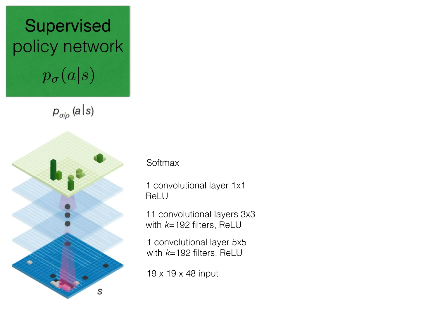
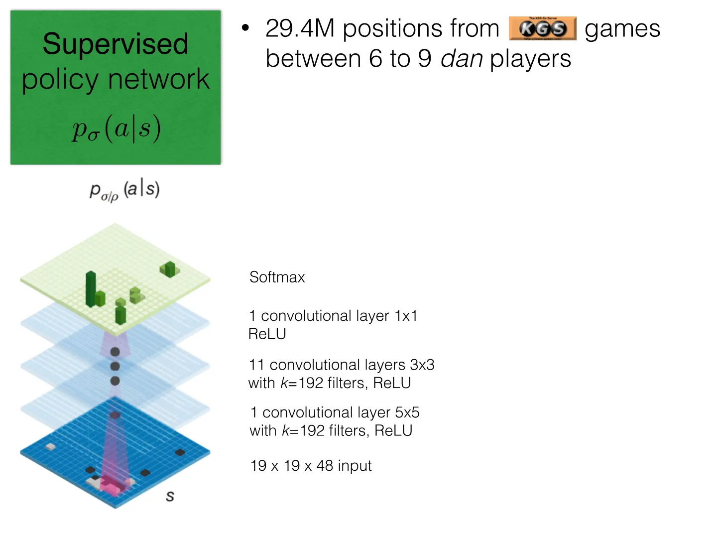
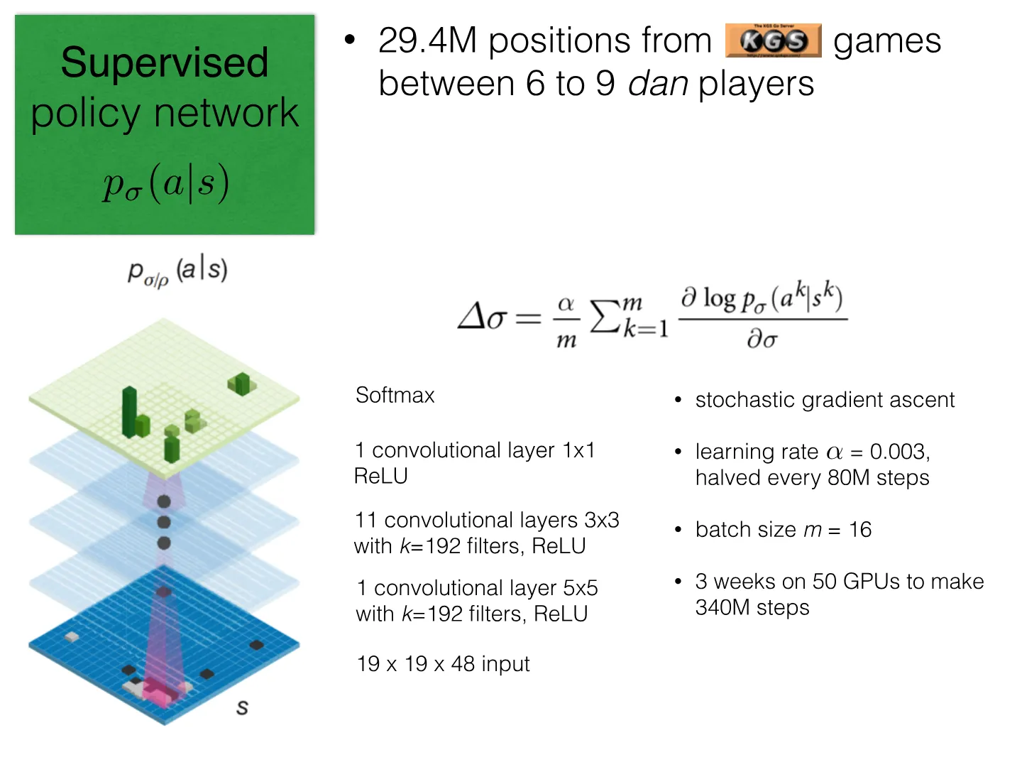
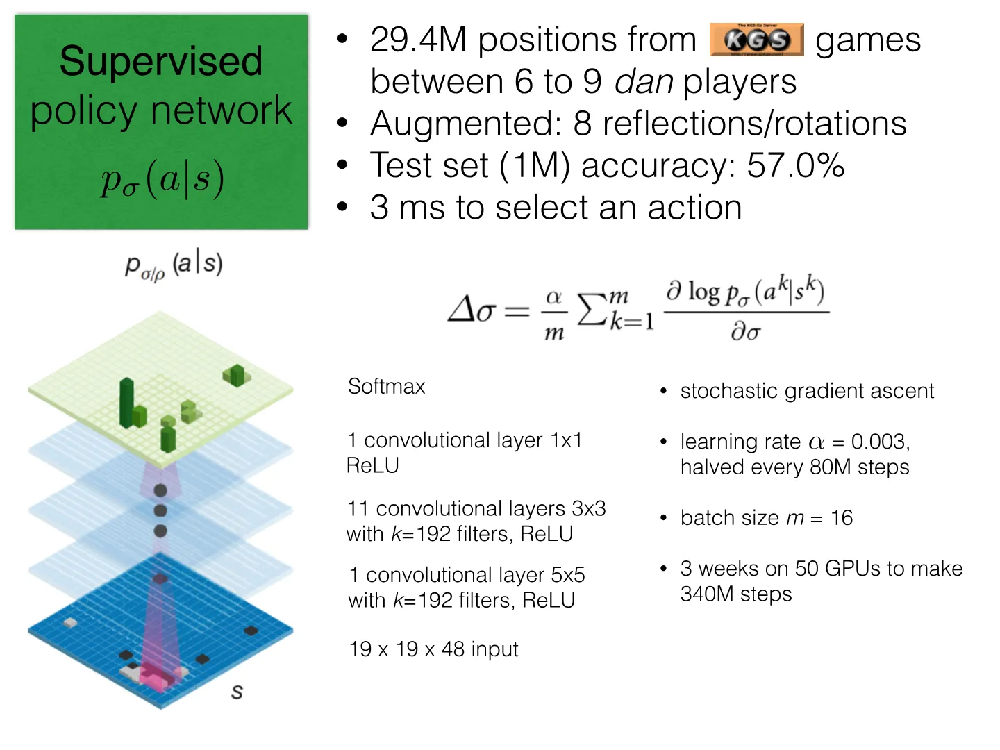
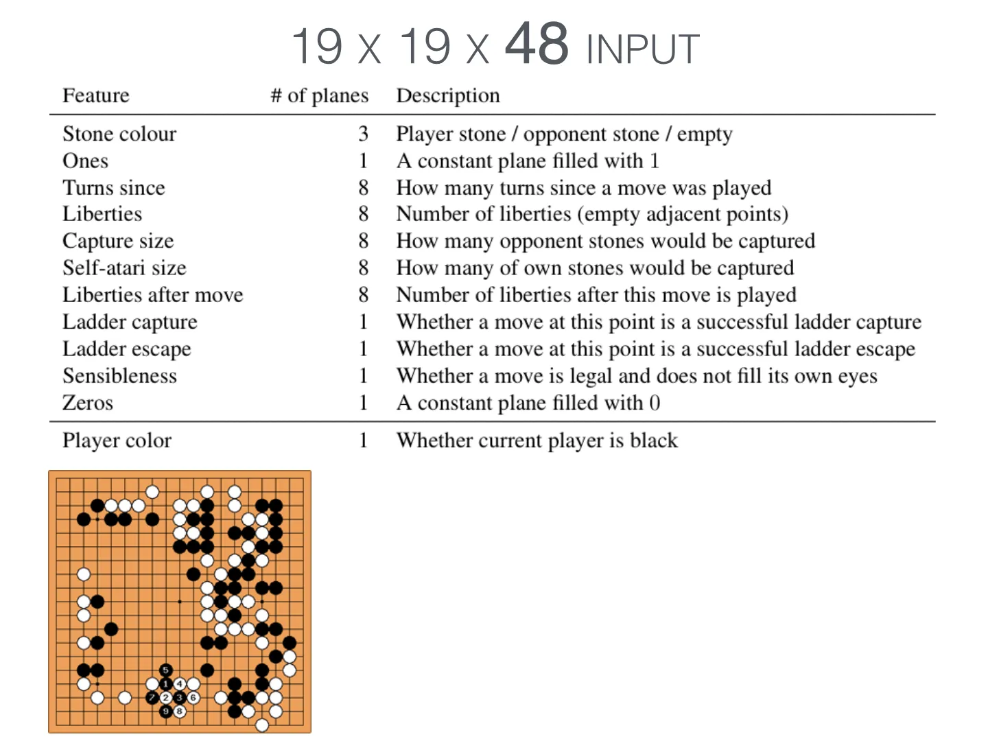
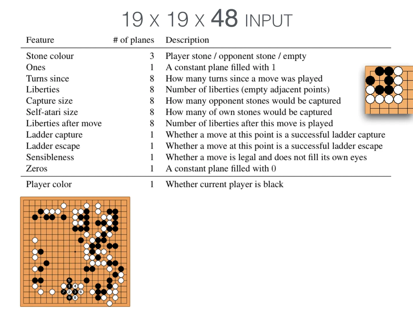
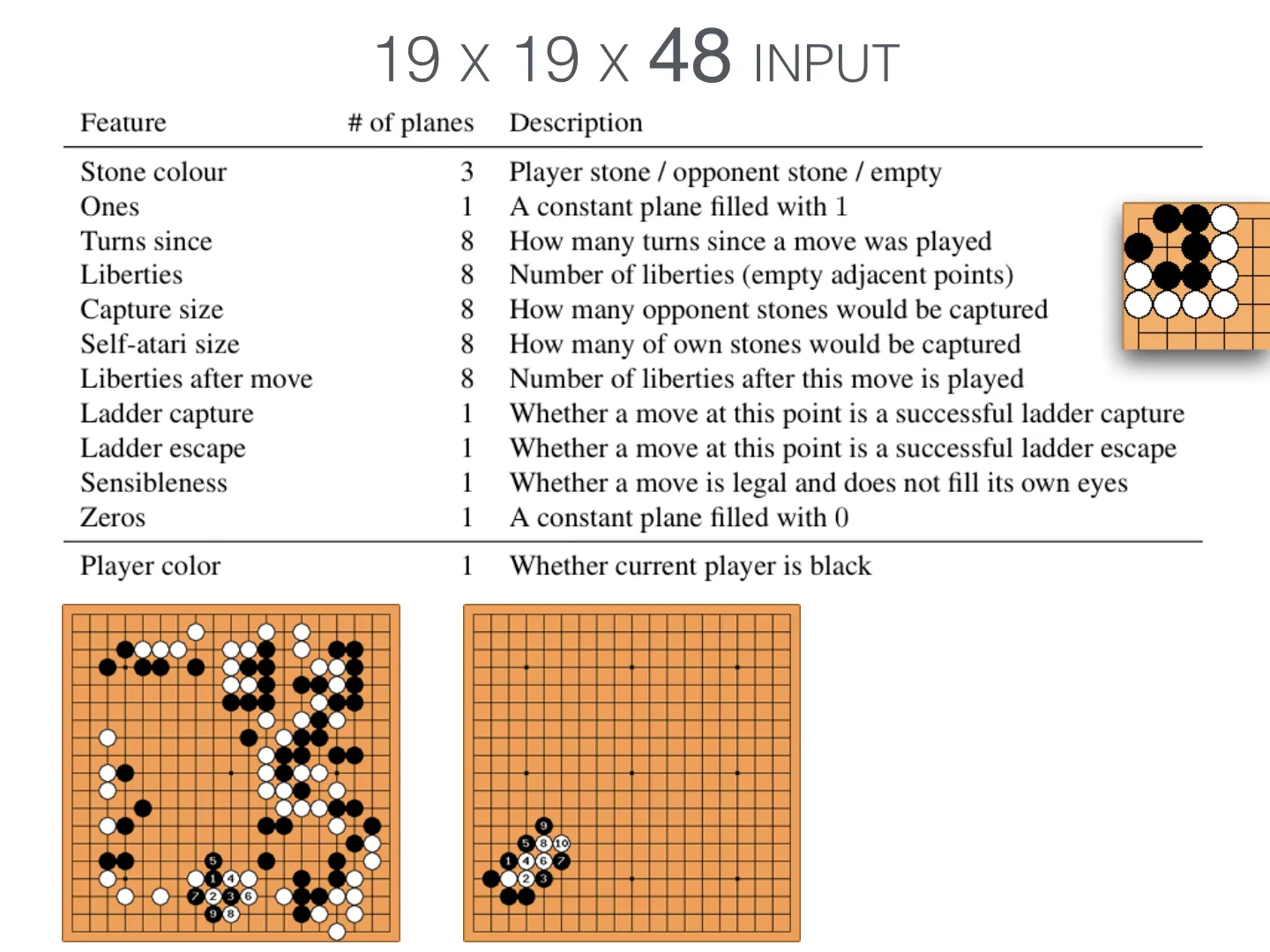
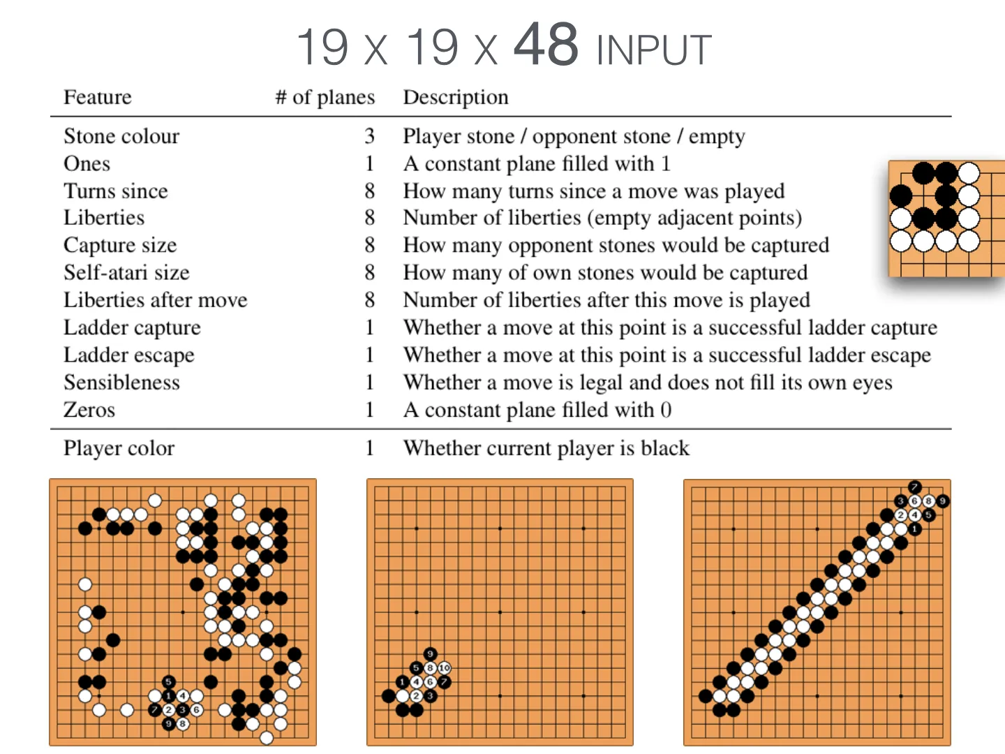
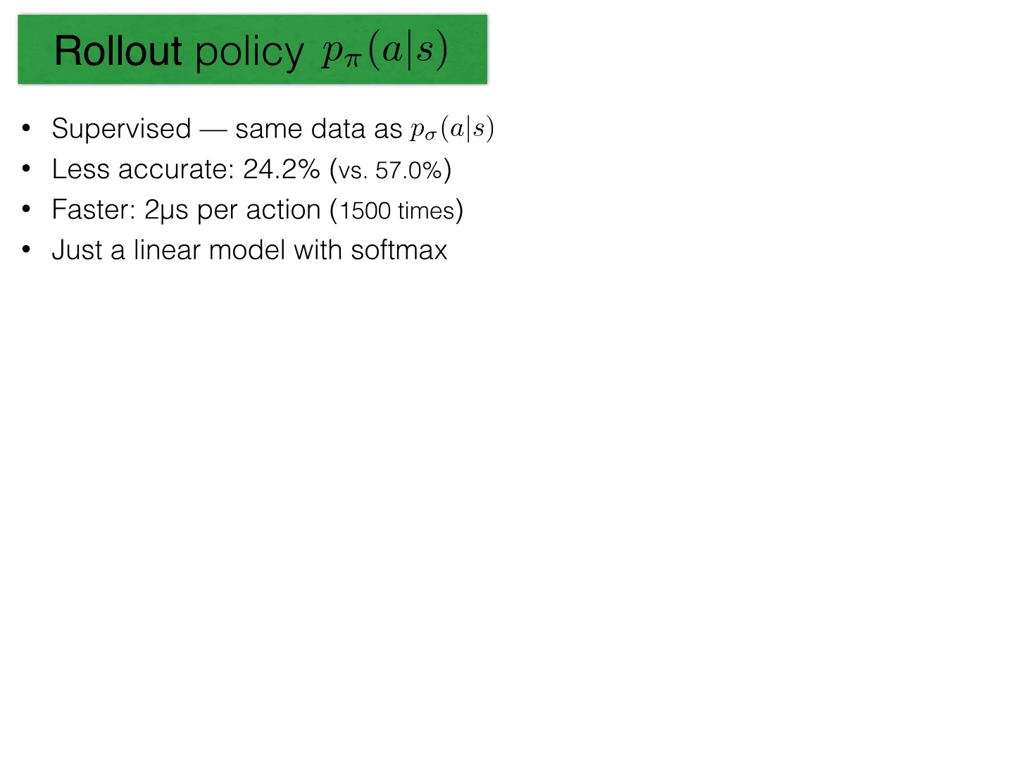
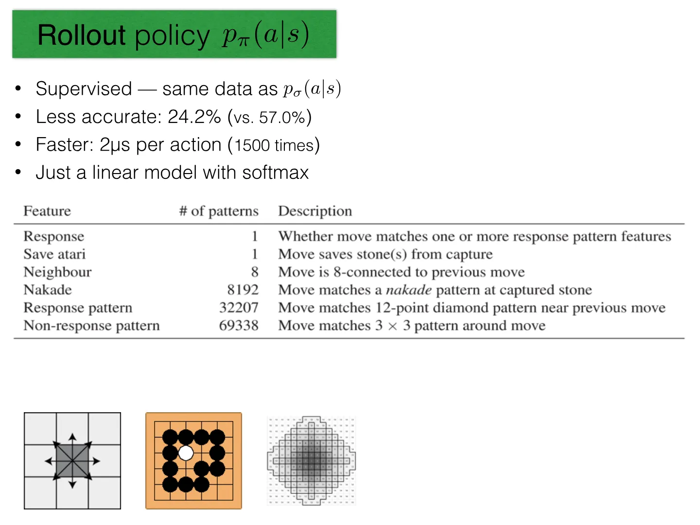
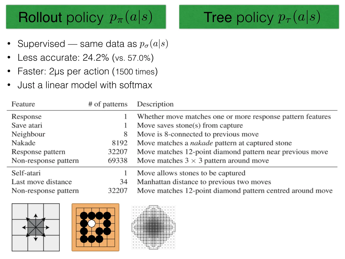
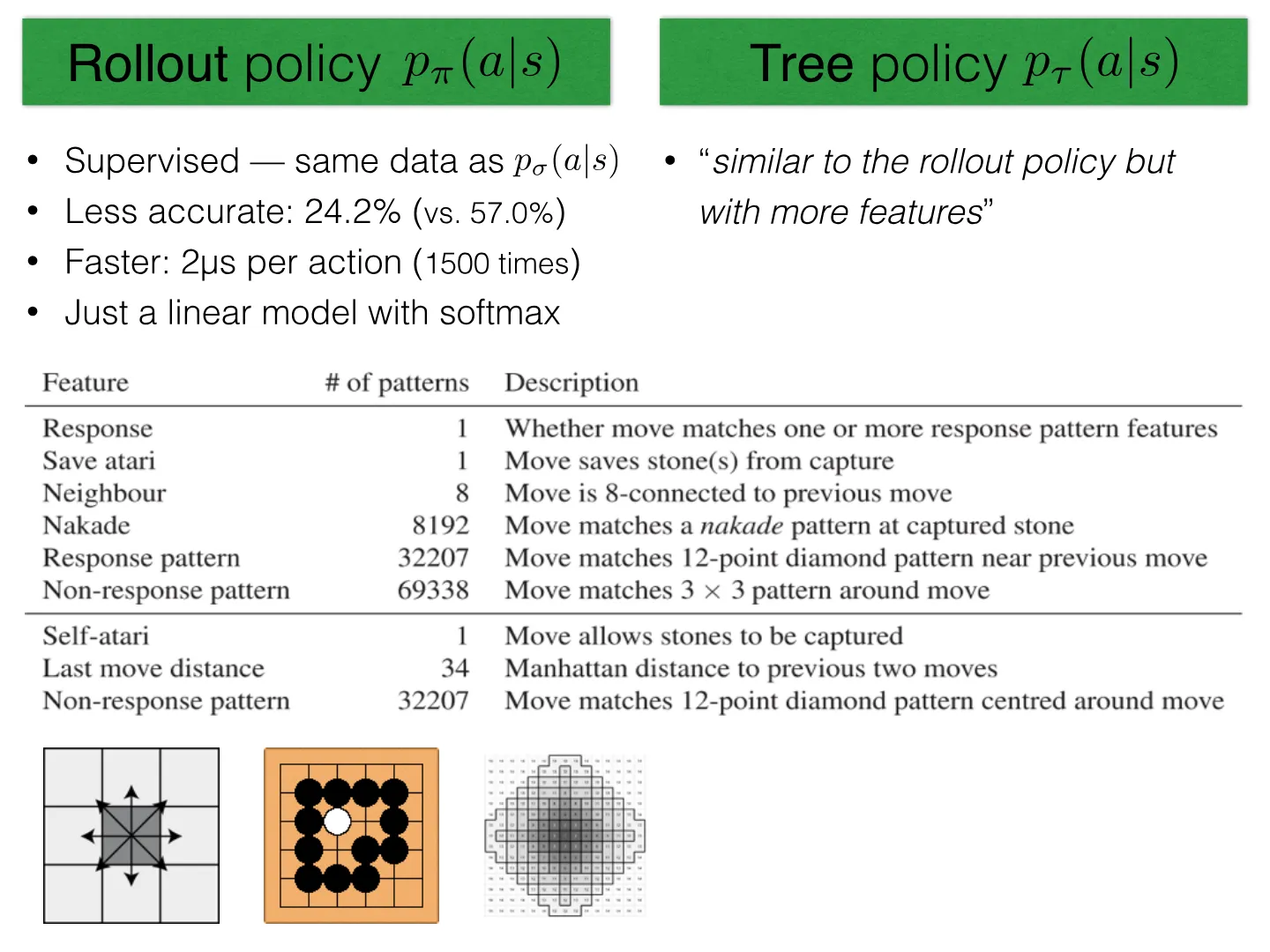
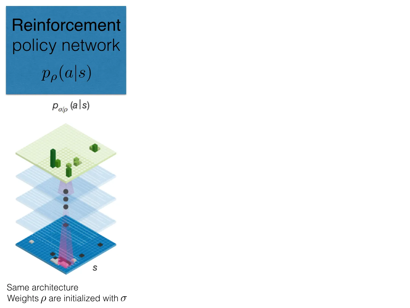
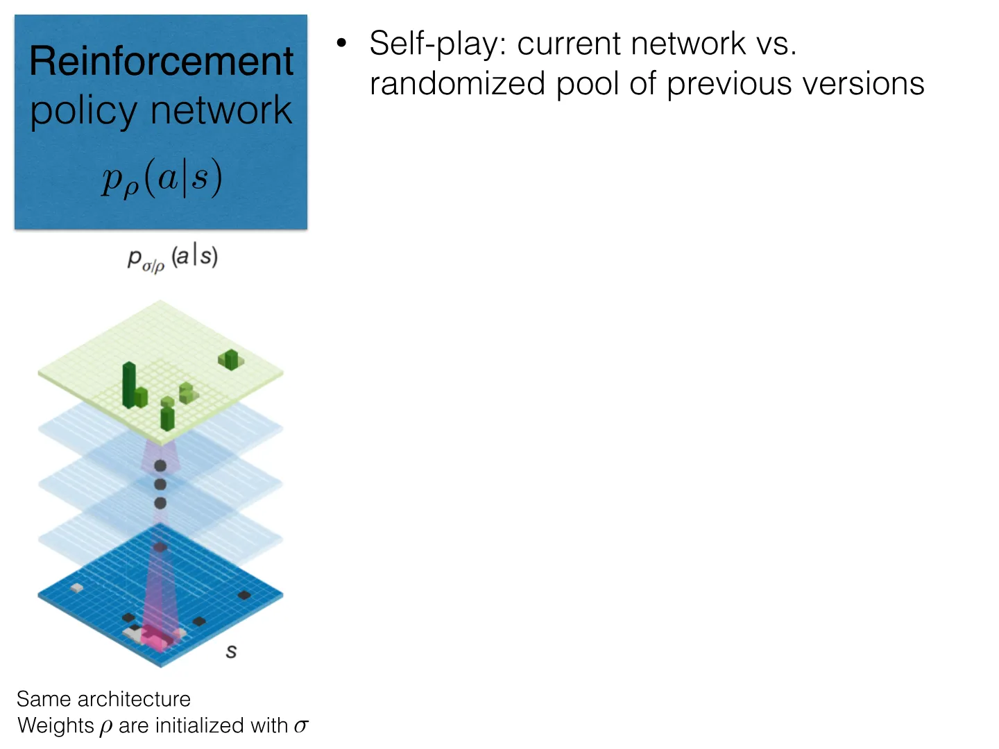
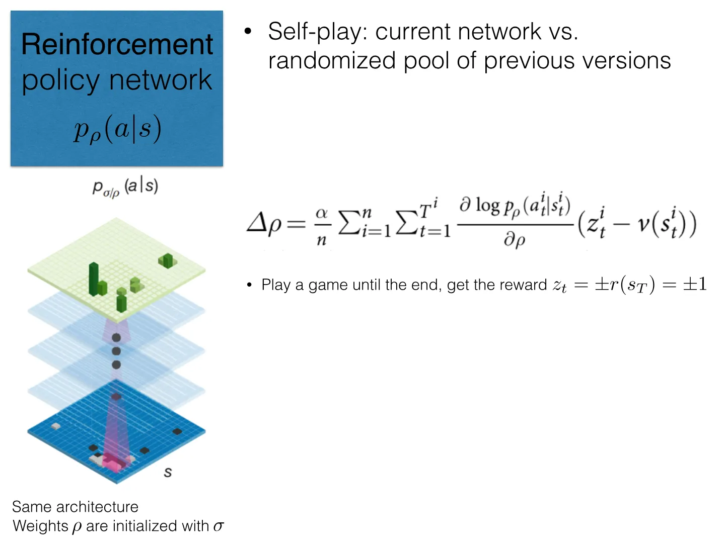
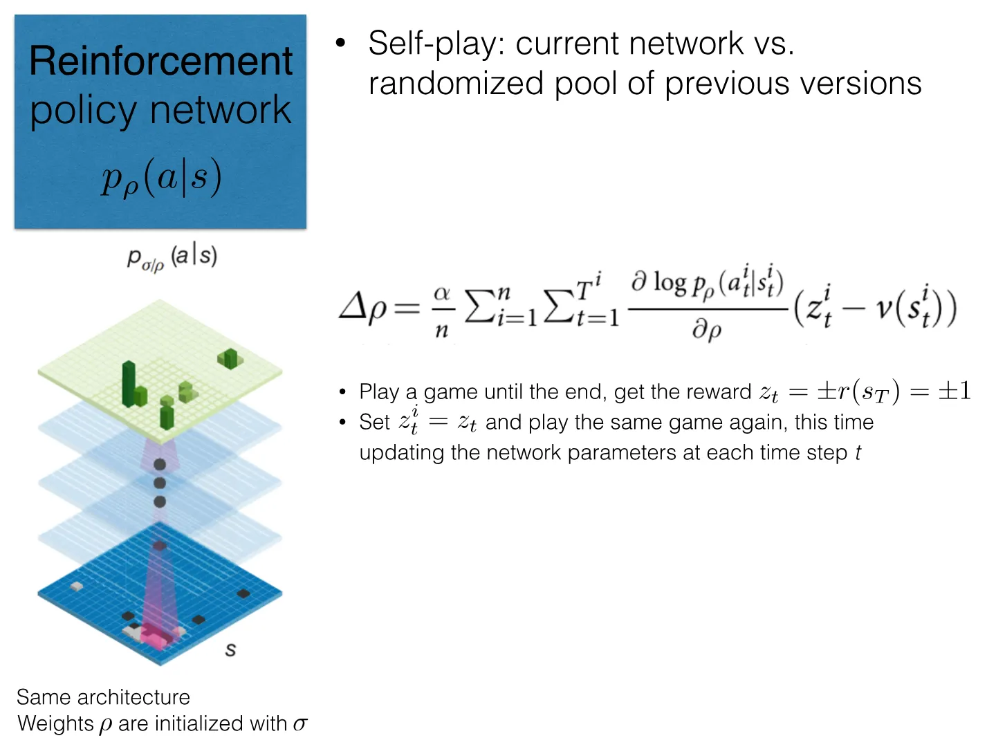
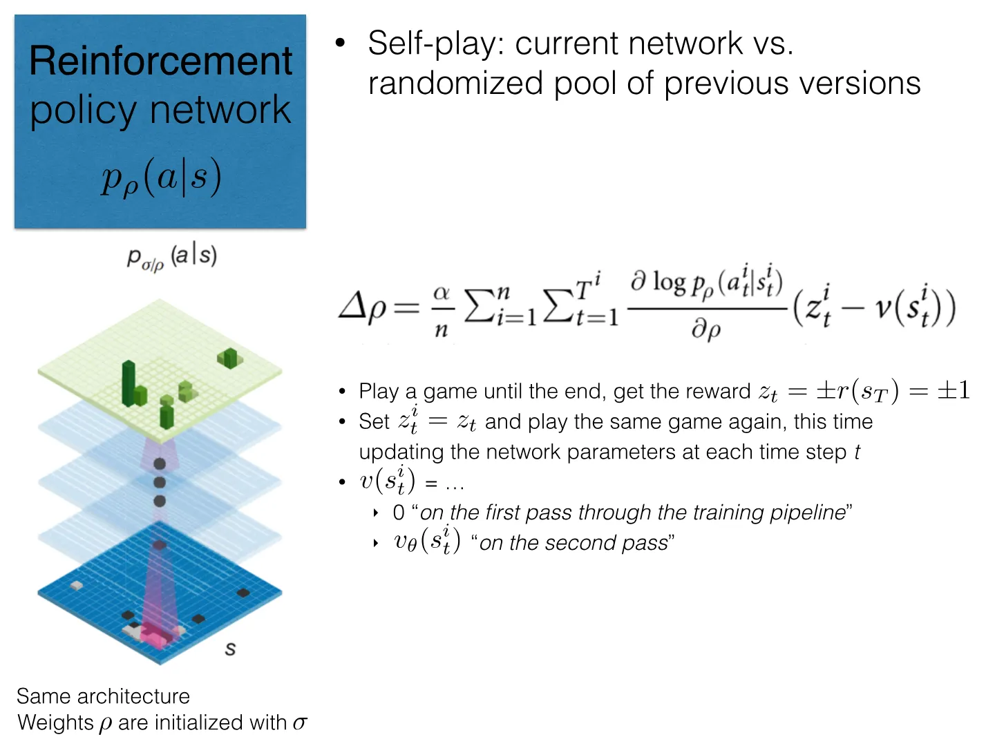
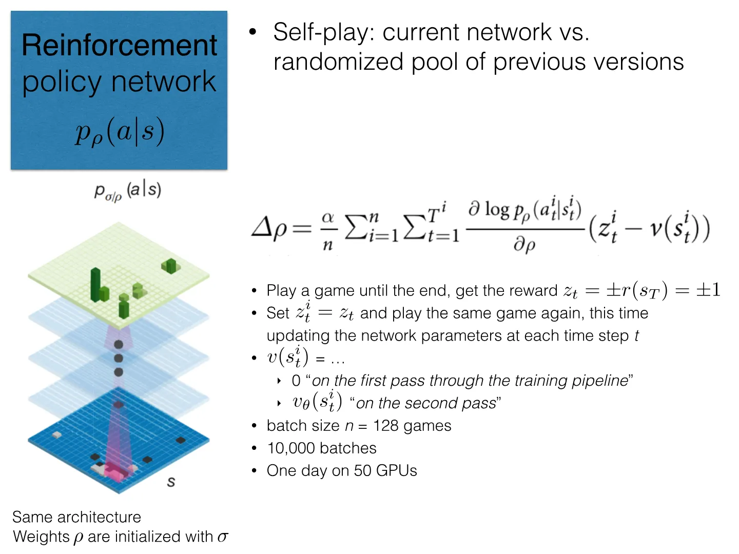
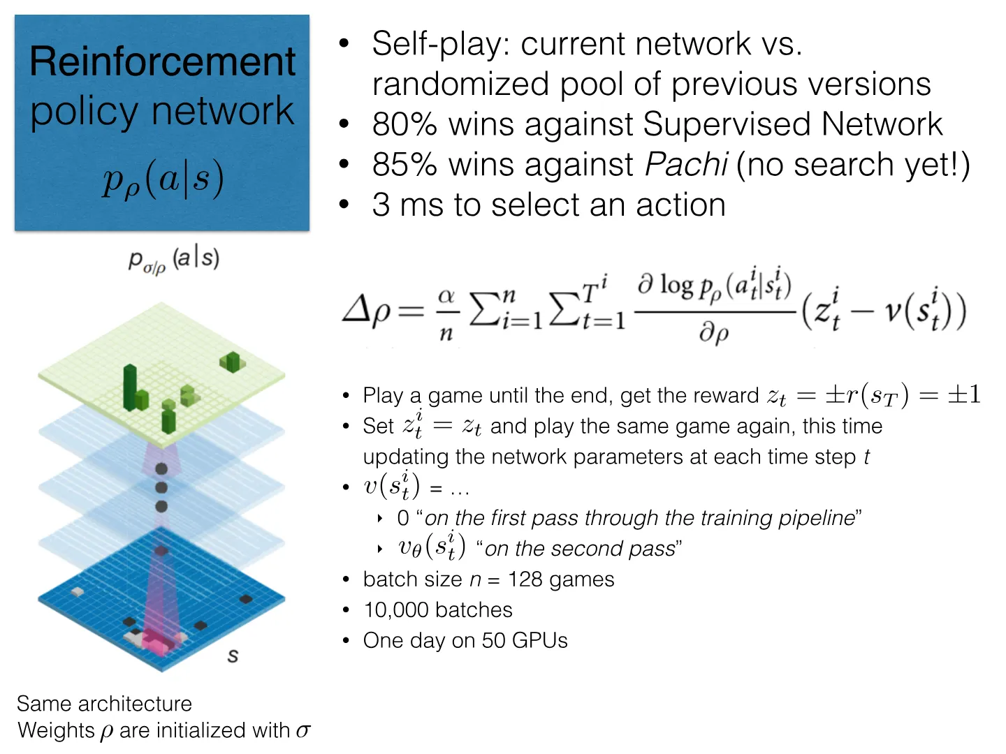
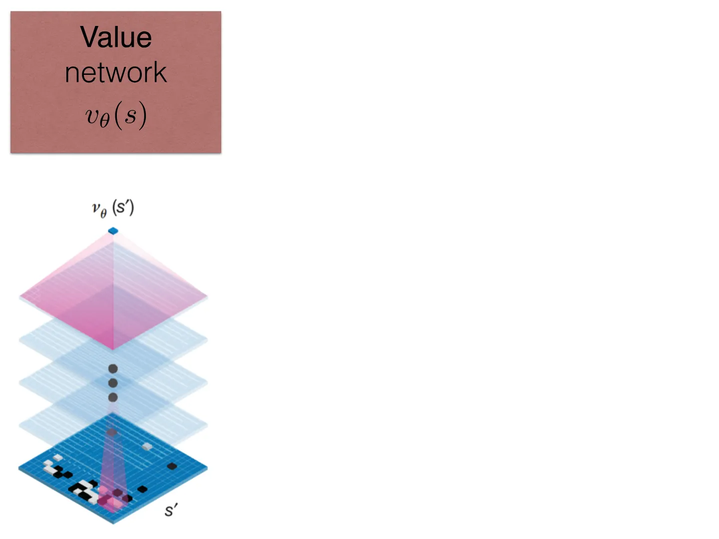
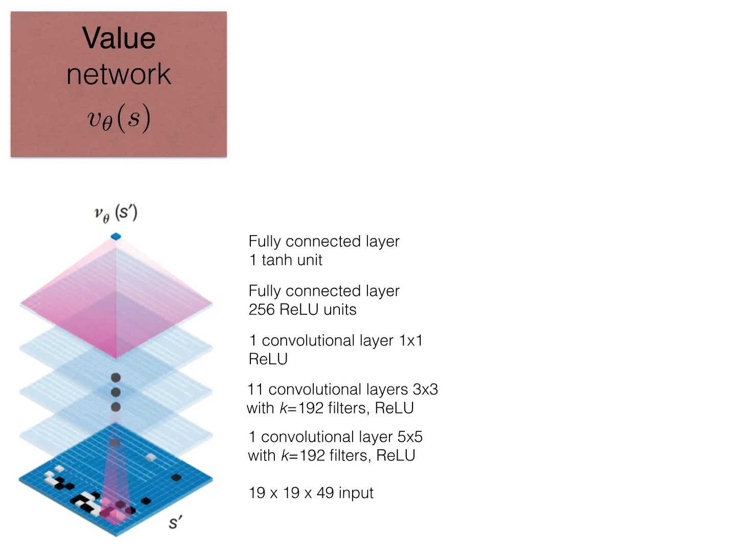
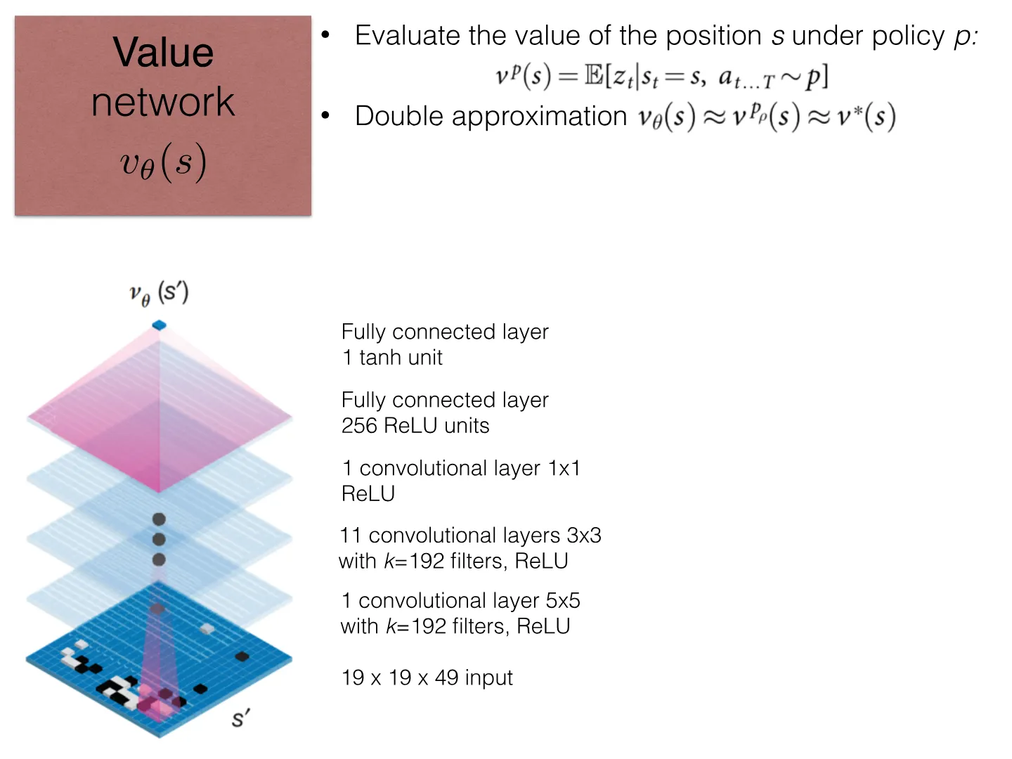
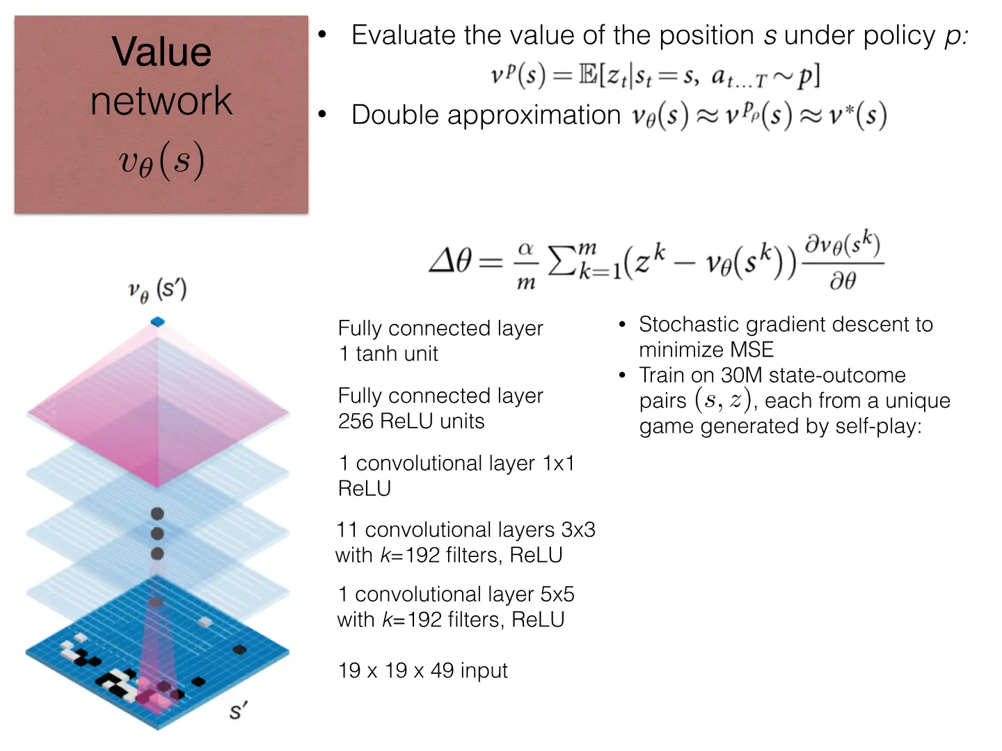
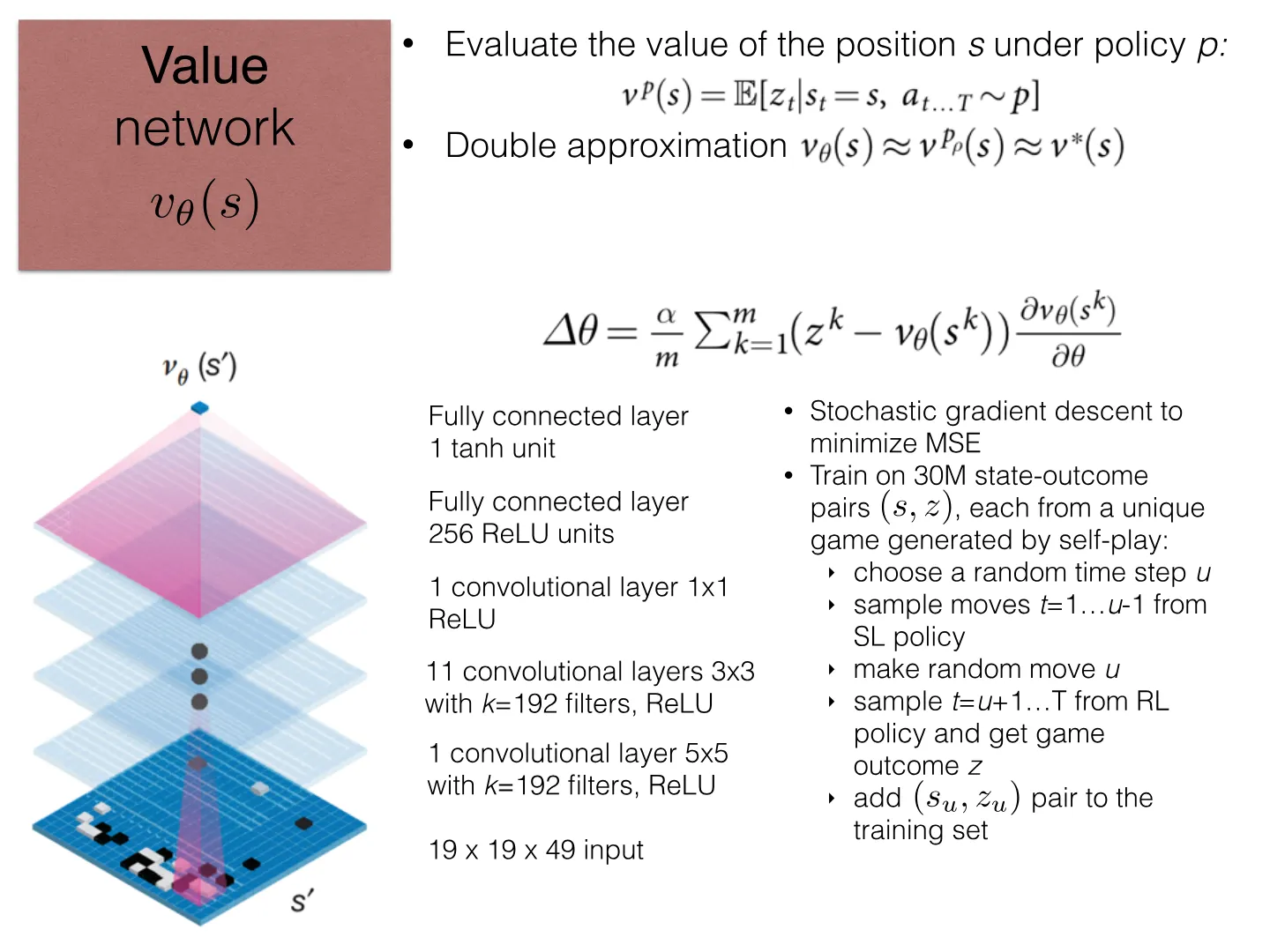
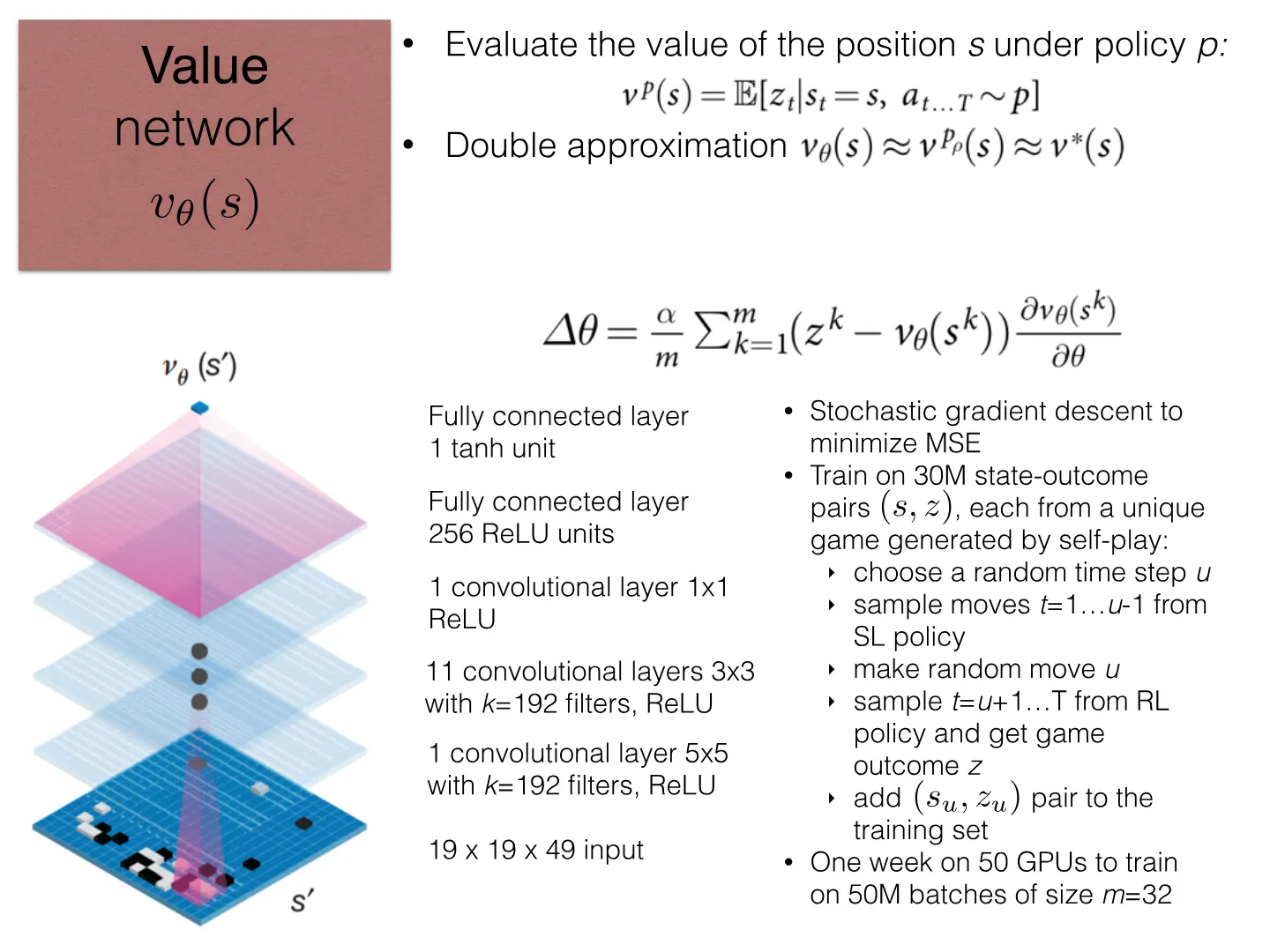
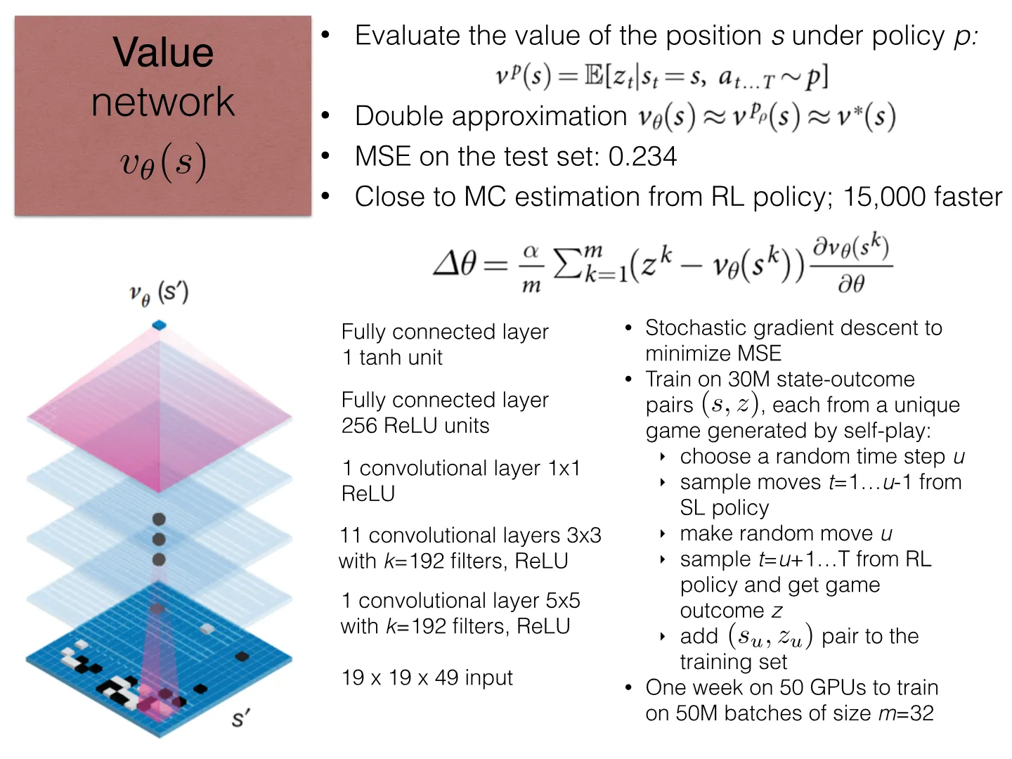
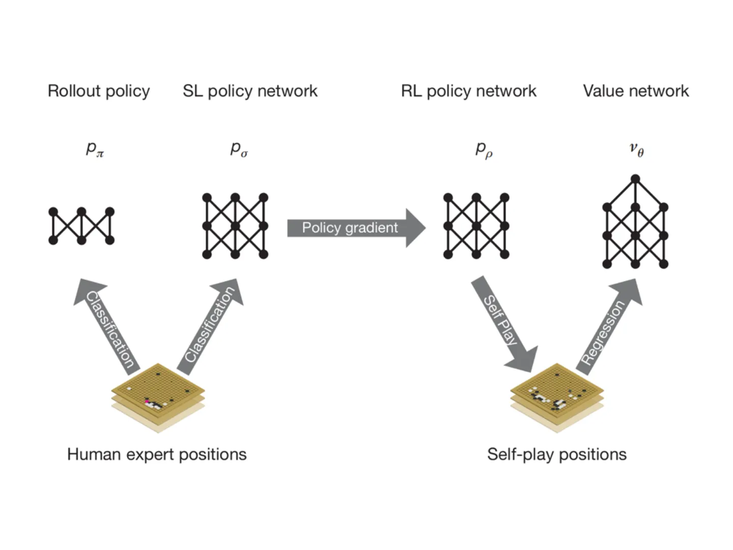
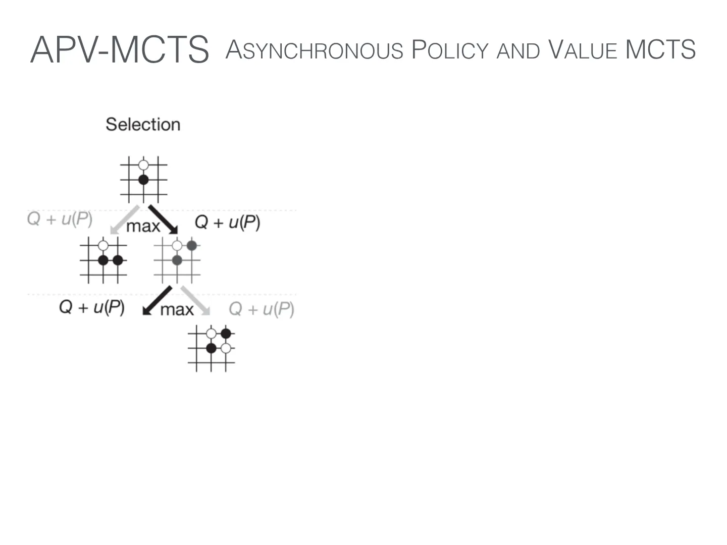
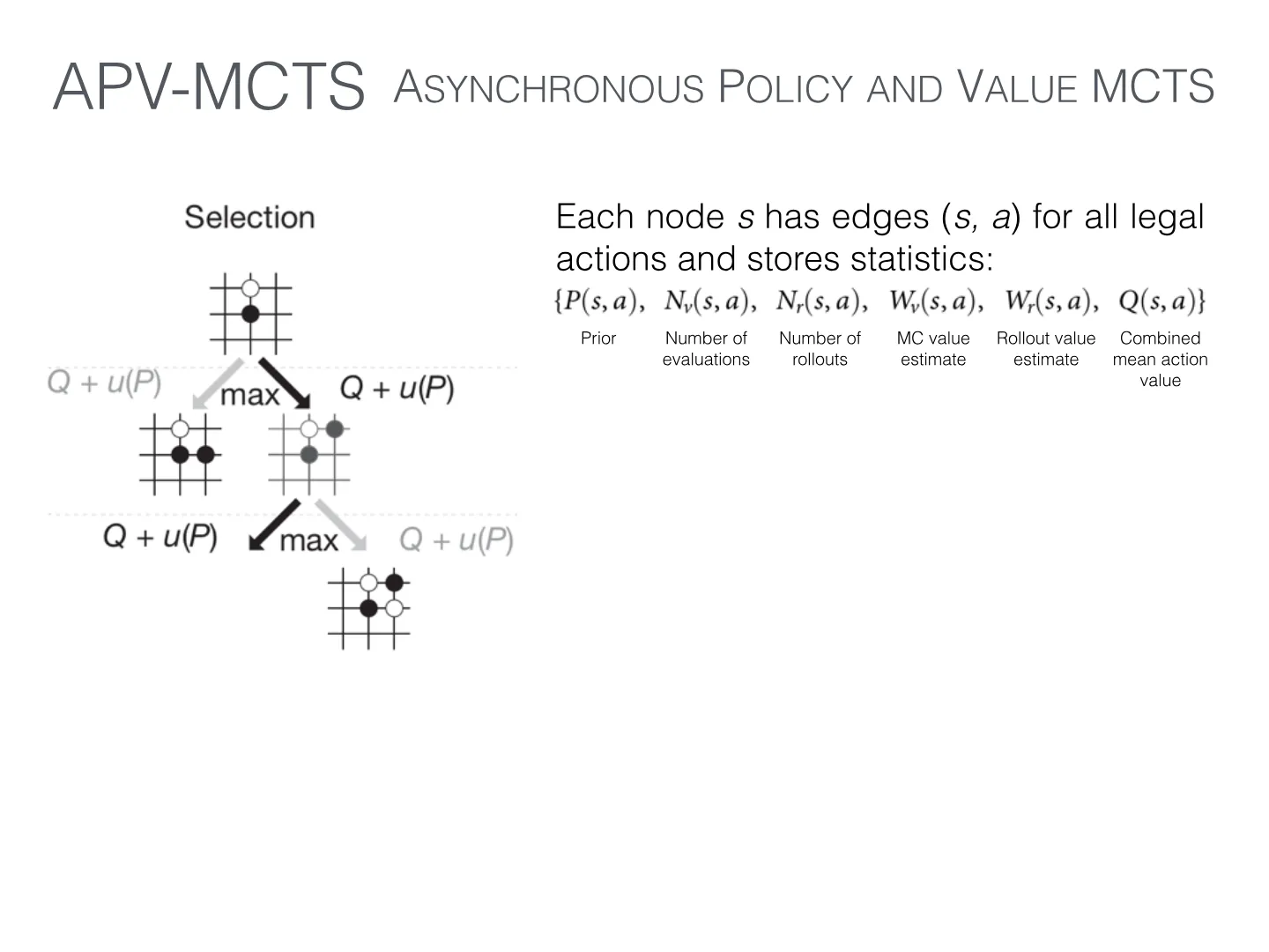
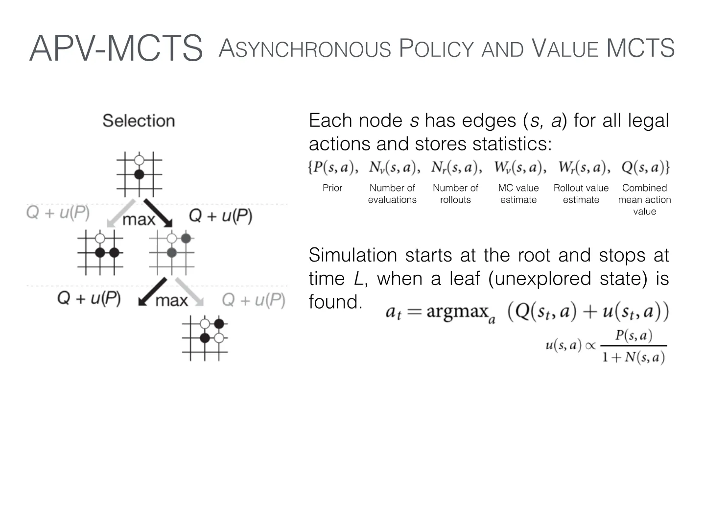
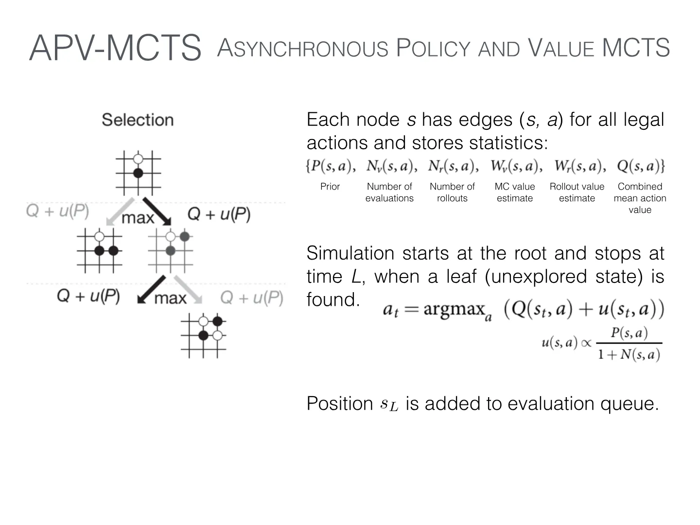
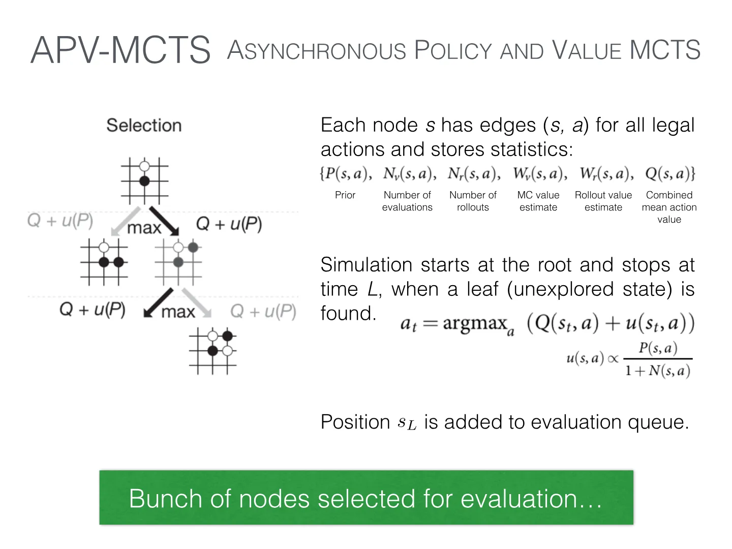
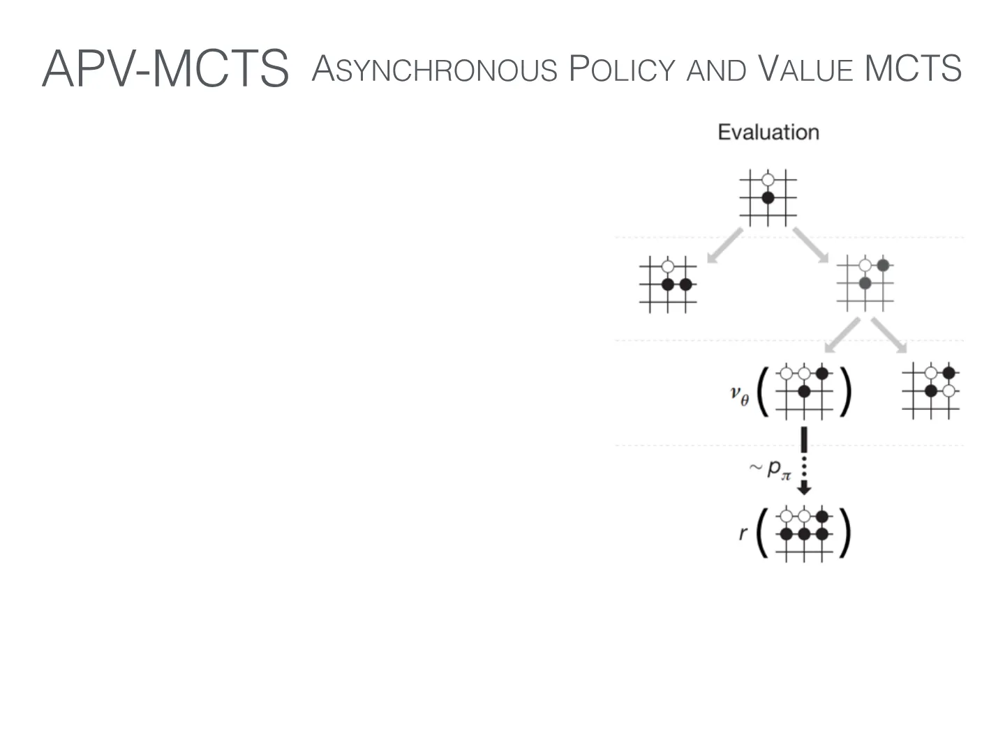
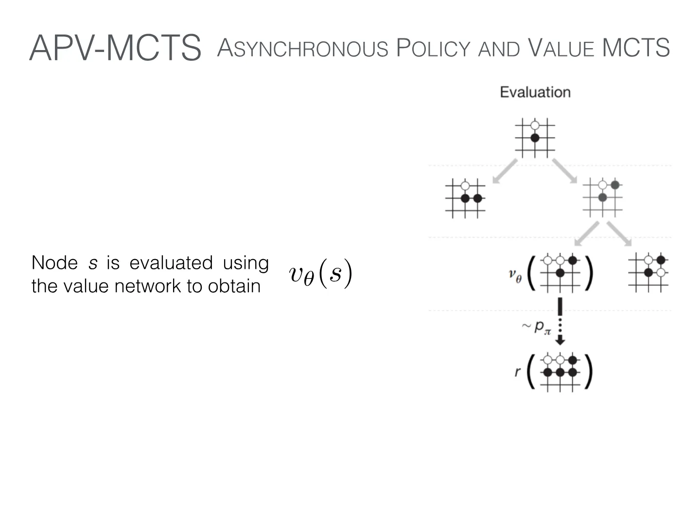
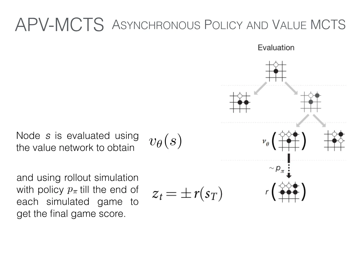
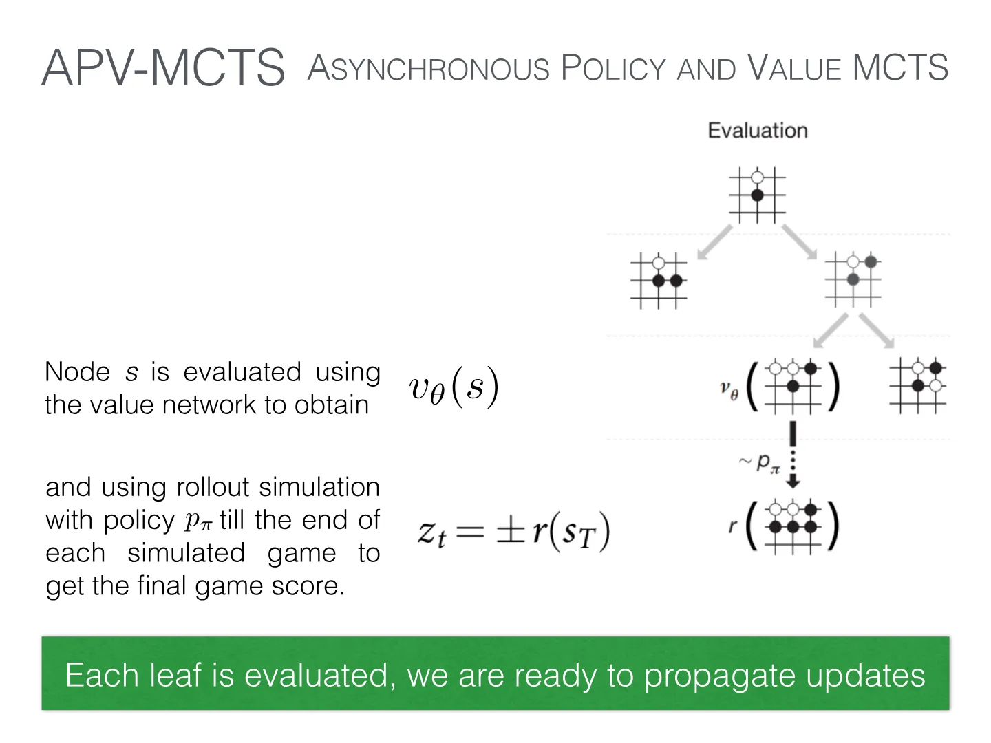
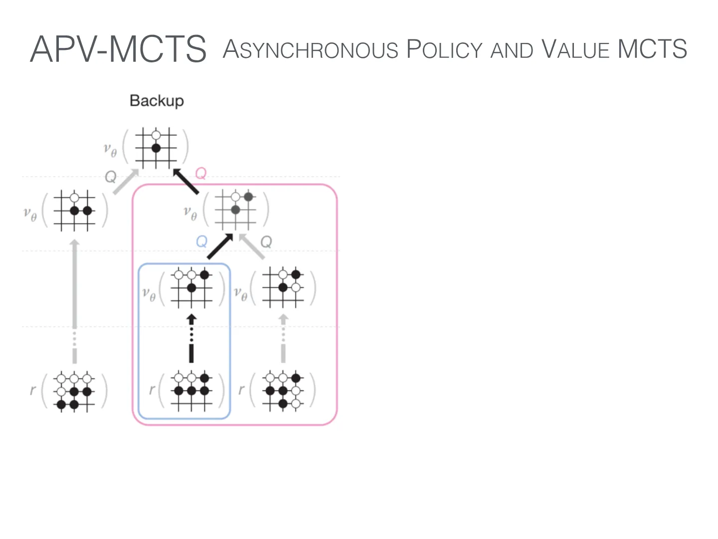
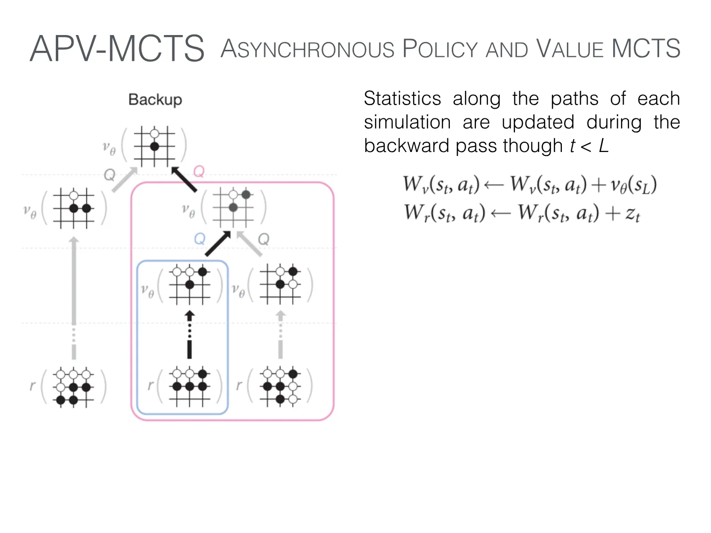
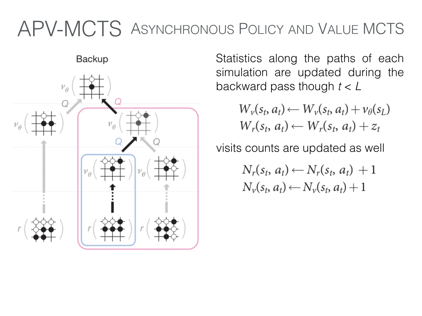
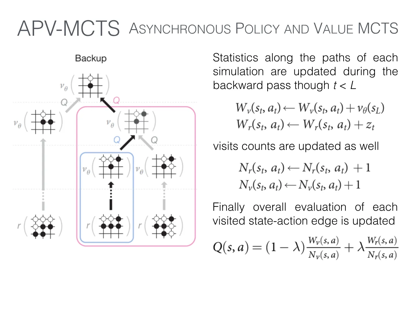
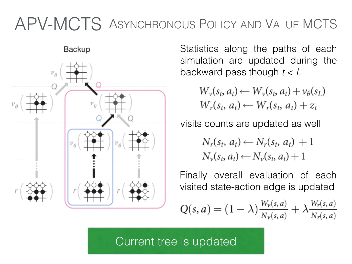
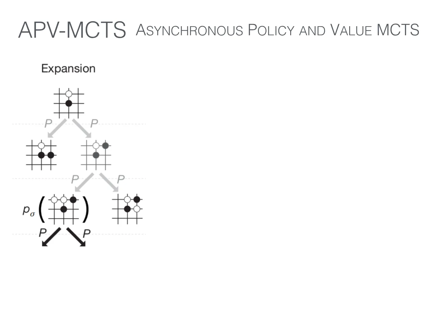
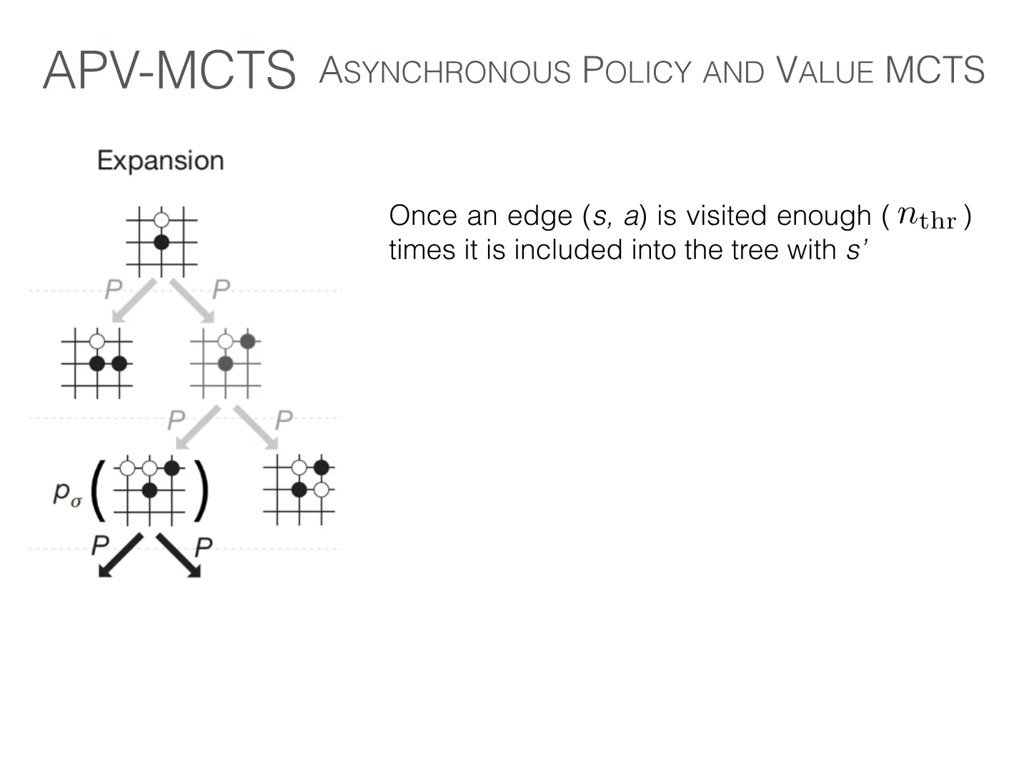
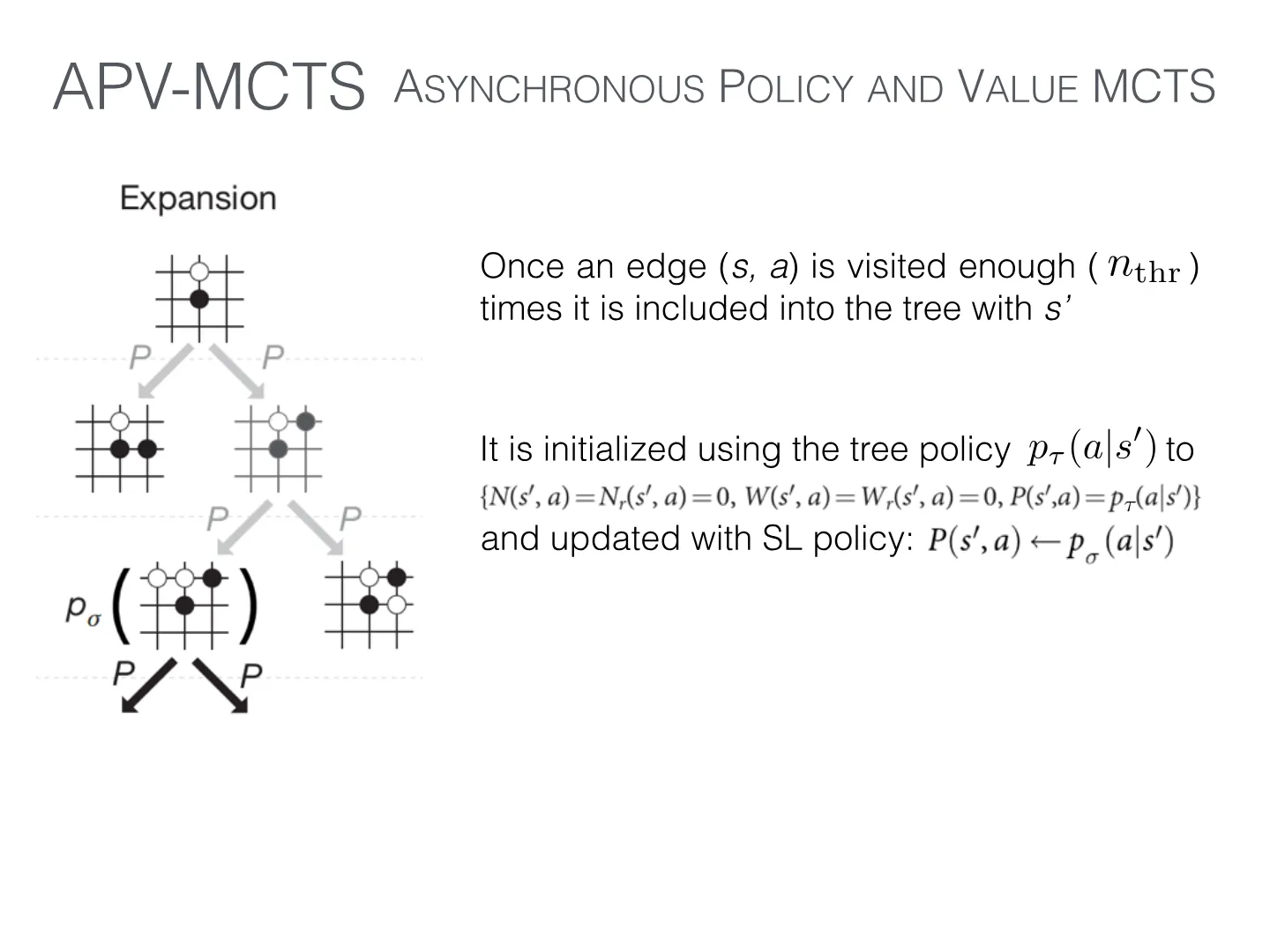
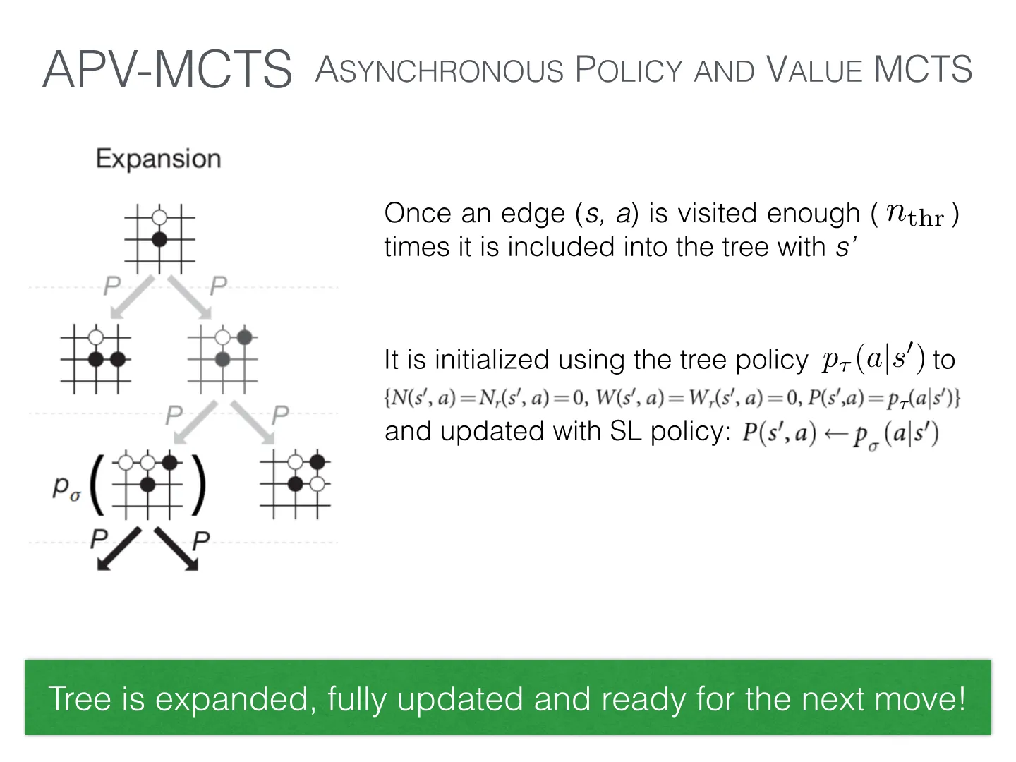
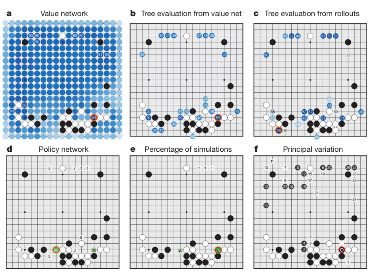
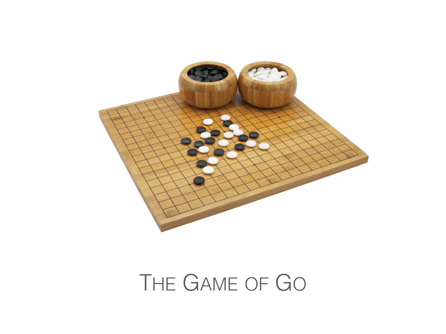
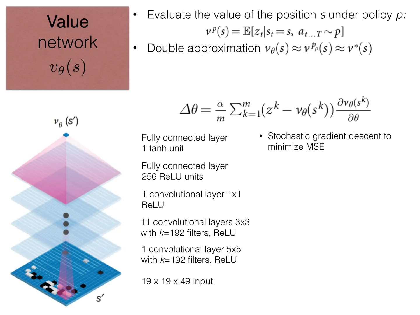
Slide 1 of 66: Article overview by Ilya Kuzovkin David Silver et al. from Google DeepMind Reinforcement Learning Seminar University of Tartu, 2016 Mastering the game of Go with deep neural networks and tree searchSlide 2 of 66: THE GAME OF GOSlide 3 of 66: BOARDSlide 4 of 66: BOARD STONESSlide 5 of 66: BOARD STONES GROUPSSlide 6 of 66: BOARD STONES LIBERTIES GROUPSSlide 7 of 66: BOARD STONES LIBERTIES CAPTURE GROUPSSlide 8 of 66: BOARD STONES LIBERTIES CAPTURE KO GROUPSSlide 9 of 66: BOARD STONES LIBERTIES CAPTURE KO GROUPS EXAMPLESSlide 10 of 66: BOARD STONES LIBERTIES CAPTURE KO GROUPS EXAMPLESSlide 11 of 66: BOARD STONES LIBERTIES CAPTURE KO GROUPS EXAMPLESSlide 12 of 66: BOARD STONES LIBERTIES CAPTURE TWO EYES KO GROUPS EXAMPLESSlide 13 of 66: BOARD STONES LIBERTIES CAPTURE FINAL COUNT KO GROUPS EXAMPLES TWO EYESSlide 14 of 66: TRAININGSlide 15 of 66: Supervised policy network p � ( a | s ) Reinforcement policy network p ⇢ ( a | s ) Rollout policy network p ⇡ ( a | s ) Value ! network v ✓ ( s ) Tree policy network p ⌧ ( a | s ) TRAINING THE BUILDING BLOCKS SUPERVISED CLASSIFICATION REINFORCEMENT SUPERVISED REGRESSIONSlide 16 of 66: Supervised policy network p � ( a | s )Slide 17 of 66: Supervised policy network p � ( a | s ) 19 x 19 x 48 input 1 convolutional layer 5x5 with k =192 filters, ReLU 11 convolutional layers 3x3 with k =192 filters, ReLU 1 convolutional layer 1x1 ReLU SoftmaxSlide 18 of 66: Supervised policy network p � ( a | s ) 19 x 19 x 48 input 1 convolutional layer 5x5 with k =192 filters, ReLU 11 convolutional layers 3x3 with k =192 filters, ReLU Softmax 1 convolutional layer 1x1 ReLU • 29.4M positions from games between 6 to 9 dan playersSlide 19 of 66: Supervised policy network p � ( a | s ) 19 x 19 x 48 input 1 convolutional layer 5x5 with k =192 filters, ReLU 11 convolutional layers 3x3 with k =192 filters, ReLU Softmax • stochastic gradient ascent ! • learning rate = 0.003, halved every 80M steps ! • batch size m = 16 ! • 3…Slide 20 of 66: Supervised policy network p � ( a | s ) 19 x 19 x 48 input 1 convolutional layer 5x5 with k =192 filters, ReLU 11 convolutional layers 3x3 with k =192 filters, ReLU Softmax • stochastic gradient ascent ! • learning rate = 0.003, halved every 80M steps ! • batch size m = 16 ! • 3…Slide 21 of 66: 19 X 19 X 48 INPUTSlide 22 of 66: 19 X 19 X 48 INPUTSlide 23 of 66: 19 X 19 X 48 INPUTSlide 24 of 66: 19 X 19 X 48 INPUTSlide 25 of 66: Rollout policy p ⇡ ( a | s ) • Supervised — same data as • Less accurate: 24.2% (vs. 57.0%) • Faster: 2 μ s per action (1500 times) • Just a linear model with softmax p � ( a | s )Slide 26 of 66: Rollout policy p ⇡ ( a | s ) • Supervised — same data as • Less accurate: 24.2% (vs. 57.0%) • Faster: 2 μ s per action (1500 times) • Just a linear model with softmax p � ( a | s )Slide 27 of 66: Rollout policy p ⇡ ( a | s ) Tree policy p ⌧ ( a | s ) • Supervised — same data as • Less accurate: 24.2% (vs. 57.0%) • Faster: 2 μ s per action (1500 times) • Just a linear model with softmax p � ( a | s )Slide 28 of 66: Rollout policy p ⇡ ( a | s ) • “ similar to the rollout policy but with more features ” Tree policy p ⌧ ( a | s ) • Supervised — same data as • Less accurate: 24.2% (vs. 57.0%) • Faster: 2 μ s per action (1500 times) • Just a linear model with softmax p � ( a | s )Slide 29 of 66: Reinforcement policy network p ⇢ ( a | s ) Same architecture Weights are initialized with ⇢ �Slide 30 of 66: Reinforcement policy network p ⇢ ( a | s ) Same architecture Weights are initialized with ⇢ � • Self-play: current network vs. randomized pool of previous versionsSlide 31 of 66: Reinforcement policy network p ⇢ ( a | s ) Same architecture Weights are initialized with ⇢ � • Self-play: current network vs. randomized pool of previous versions • Play a game until the end, get the reward z t = ± r ( s T ) = ± 1Slide 32 of 66: Reinforcement policy network p ⇢ ( a | s ) Same architecture Weights are initialized with ⇢ � • Self-play: current network vs. randomized pool of previous versions • Play a game until the end, get the reward • Set and play the same game again, this time updating the network…Slide 33 of 66: Reinforcement policy network p ⇢ ( a | s ) Same architecture Weights are initialized with ⇢ � • Self-play: current network vs. randomized pool of previous versions • Play a game until the end, get the reward • Set and play the same game again, this time updating the network…Slide 34 of 66: Reinforcement policy network p ⇢ ( a | s ) Same architecture Weights are initialized with ⇢ � • Self-play: current network vs. randomized pool of previous versions • Play a game until the end, get the reward • Set and play the same game again, this time updating the network…Slide 35 of 66: Reinforcement policy network p ⇢ ( a | s ) Same architecture Weights are initialized with ⇢ � • Self-play: current network vs. randomized pool of previous versions • 80% wins against Supervised Network • 85% wins against Pachi (no search yet!) • 3 ms to select an action • Play a…Slide 36 of 66: Value ! network v ✓ ( s )Slide 37 of 66: 19 x 19 x 49 input 1 convolutional layer 5x5 with k =192 filters, ReLU 11 convolutional layers 3x3 with k =192 filters, ReLU Fully connected layer 256 ReLU units Value ! network v ✓ ( s ) Fully connected layer 1 tanh unit 1 convolutional layer 1x1 ReLUSlide 38 of 66: 19 x 19 x 49 input 1 convolutional layer 5x5 with k =192 filters, ReLU 11 convolutional layers 3x3 with k =192 filters, ReLU Fully connected layer 256 ReLU units Value ! network v ✓ ( s ) Fully connected layer 1 tanh unit • Evaluate the value of the position s under policy p: !…Slide 39 of 66: 19 x 19 x 49 input 1 convolutional layer 5x5 with k =192 filters, ReLU 11 convolutional layers 3x3 with k =192 filters, ReLU Fully connected layer 256 ReLU units Value ! network v ✓ ( s ) Fully connected layer 1 tanh unit • Evaluate the value of the position s under policy p: !…Slide 40 of 66: 19 x 19 x 49 input 1 convolutional layer 5x5 with k =192 filters, ReLU 11 convolutional layers 3x3 with k =192 filters, ReLU Fully connected layer 256 ReLU units Value ! network v ✓ ( s ) Fully connected layer 1 tanh unit • Evaluate the value of the position s under policy p: !…Slide 41 of 66: 19 x 19 x 49 input 1 convolutional layer 5x5 with k =192 filters, ReLU 11 convolutional layers 3x3 with k =192 filters, ReLU Fully connected layer 256 ReLU units Value ! network v ✓ ( s ) Fully connected layer 1 tanh unit • Evaluate the value of the position s under policy p: !…Slide 42 of 66: 19 x 19 x 49 input 1 convolutional layer 5x5 with k =192 filters, ReLU 11 convolutional layers 3x3 with k =192 filters, ReLU Fully connected layer 256 ReLU units Value ! network v ✓ ( s ) Fully connected layer 1 tanh unit • Evaluate the value of the position s under policy p: !…Slide 43 of 66: 19 x 19 x 49 input 1 convolutional layer 5x5 with k =192 filters, ReLU 11 convolutional layers 3x3 with k =192 filters, ReLU Fully connected layer 256 ReLU units Value ! network v ✓ ( s ) Fully connected layer 1 tanh unit • Evaluate the value of the position s under policy p: !…Slide 44 of 66Slide 45 of 66: PLAYINGSlide 46 of 66: APV-MCTS ASYNCHRONOUS POLICY AND VALUE MCTSSlide 47 of 66: APV-MCTS Each node s has edges ( s, a ) for all legal actions and stores statistics: Prior Number of evaluations Number of rollouts MC value estimate Rollout value estimate Combined mean action value ASYNCHRONOUS POLICY AND VALUE MCTSSlide 48 of 66: APV-MCTS Each node s has edges ( s, a ) for all legal actions and stores statistics: Prior Number of evaluations Number of rollouts MC value estimate Rollout value estimate Combined mean action value ASYNCHRONOUS POLICY AND VALUE MCTS Simulation starts at the root and stops at…Slide 49 of 66: APV-MCTS Each node s has edges ( s, a ) for all legal actions and stores statistics: Prior Number of evaluations Number of rollouts MC value estimate Rollout value estimate Combined mean action value ASYNCHRONOUS POLICY AND VALUE MCTS Simulation starts at the root and stops at…Slide 50 of 66: APV-MCTS Each node s has edges ( s, a ) for all legal actions and stores statistics: Prior Number of evaluations Number of rollouts MC value estimate Rollout value estimate Combined mean action value ASYNCHRONOUS POLICY AND VALUE MCTS Simulation starts at the root and stops at…Slide 51 of 66: APV-MCTS ASYNCHRONOUS POLICY AND VALUE MCTSSlide 52 of 66: APV-MCTS ASYNCHRONOUS POLICY AND VALUE MCTS Node s is evaluated using the value network to obtain v ✓ ( s )Slide 53 of 66: APV-MCTS ASYNCHRONOUS POLICY AND VALUE MCTS Node s is evaluated using the value network to obtain and using rollout simulation with policy till the end of each simulated game to get the final game score. p ⇡ ( a | s ) v ✓ ( s )Slide 54 of 66: APV-MCTS ASYNCHRONOUS POLICY AND VALUE MCTS Node s is evaluated using the value network to obtain and using rollout simulation with policy till the end of each simulated game to get the final game score. p ⇡ ( a | s ) v ✓ ( s ) Each leaf is evaluated, we are ready to propagate…Slide 55 of 66: APV-MCTS ASYNCHRONOUS POLICY AND VALUE MCTSSlide 56 of 66: APV-MCTS ASYNCHRONOUS POLICY AND VALUE MCTS Statistics along the paths of each simulation are updated during the backward pass though t < LSlide 57 of 66: APV-MCTS ASYNCHRONOUS POLICY AND VALUE MCTS Statistics along the paths of each simulation are updated during the backward pass though t < L visits counts are updated as wellSlide 58 of 66: APV-MCTS ASYNCHRONOUS POLICY AND VALUE MCTS Statistics along the paths of each simulation are updated during the backward pass though t < L visits counts are updated as well Finally overall evaluation of each visited state-action edge is updatedSlide 59 of 66: APV-MCTS ASYNCHRONOUS POLICY AND VALUE MCTS Statistics along the paths of each simulation are updated during the backward pass though t < L visits counts are updated as well Finally overall evaluation of each visited state-action edge is updated Current tree is updatedSlide 60 of 66: APV-MCTS ASYNCHRONOUS POLICY AND VALUE MCTSSlide 61 of 66: APV-MCTS ASYNCHRONOUS POLICY AND VALUE MCTS Once an edge ( s, a ) is visited enough ( ) times it is included into the tree with s’ n thrSlide 62 of 66: APV-MCTS ASYNCHRONOUS POLICY AND VALUE MCTS Once an edge ( s, a ) is visited enough ( ) times it is included into the tree with s’ n thr It is initialized using the tree policy to and updated with SL policy: p ⌧ ( a | s 0 ) ⌧Slide 63 of 66: APV-MCTS ASYNCHRONOUS POLICY AND VALUE MCTS Tree is expanded, fully updated and ready for the next move! Once an edge ( s, a ) is visited enough ( ) times it is included into the tree with s’ n thr It is initialized using the tree policy to and updated with SL policy: p ⌧ ( a |…Slide 64 of 66Slide 65 of 66: https://www.youtube.com/watch?v=oRvlyEpOQ-8 WINNINGSlide 66 of 66: https://www.youtube.com/watch?v=oRvlyEpOQ-8
1 / 66

Mastering the game of Go with deep neural networks and tree search (article overview)
A talk given at the Reinforcement Learning Seminar @ University of Tartu — going through the details of how the AlphaGo system works.
Download PDF