machine learning, ai, cs · slides · talks & lectures

Introduction to Machine Learning @ Mooncascade ML Camp
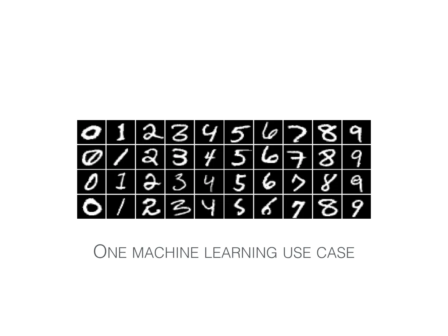
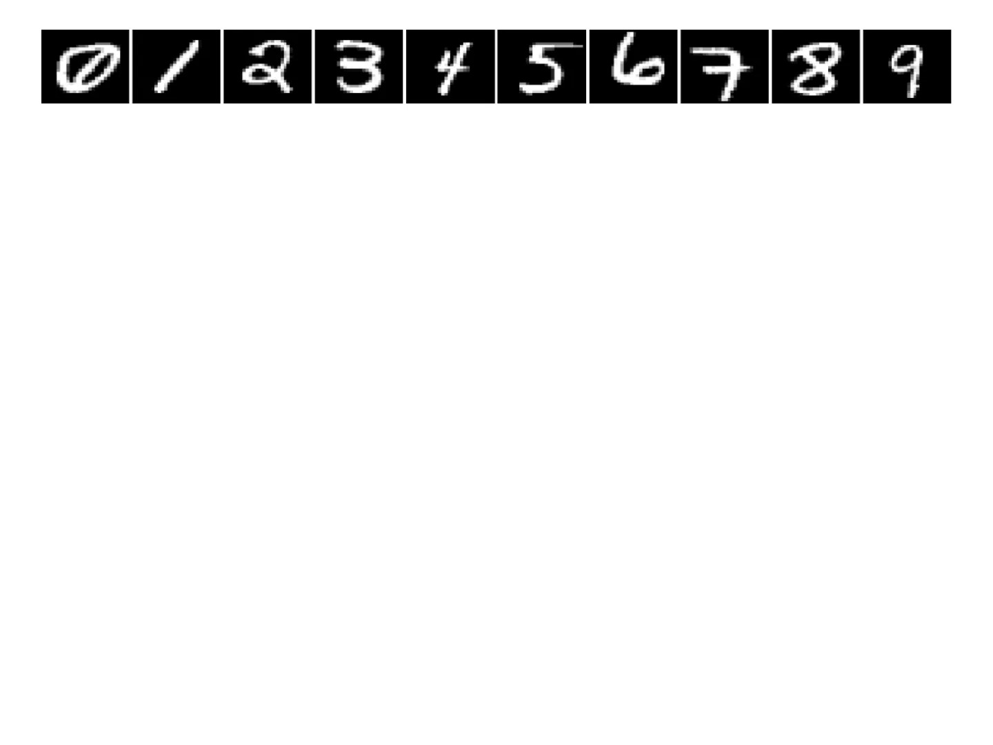
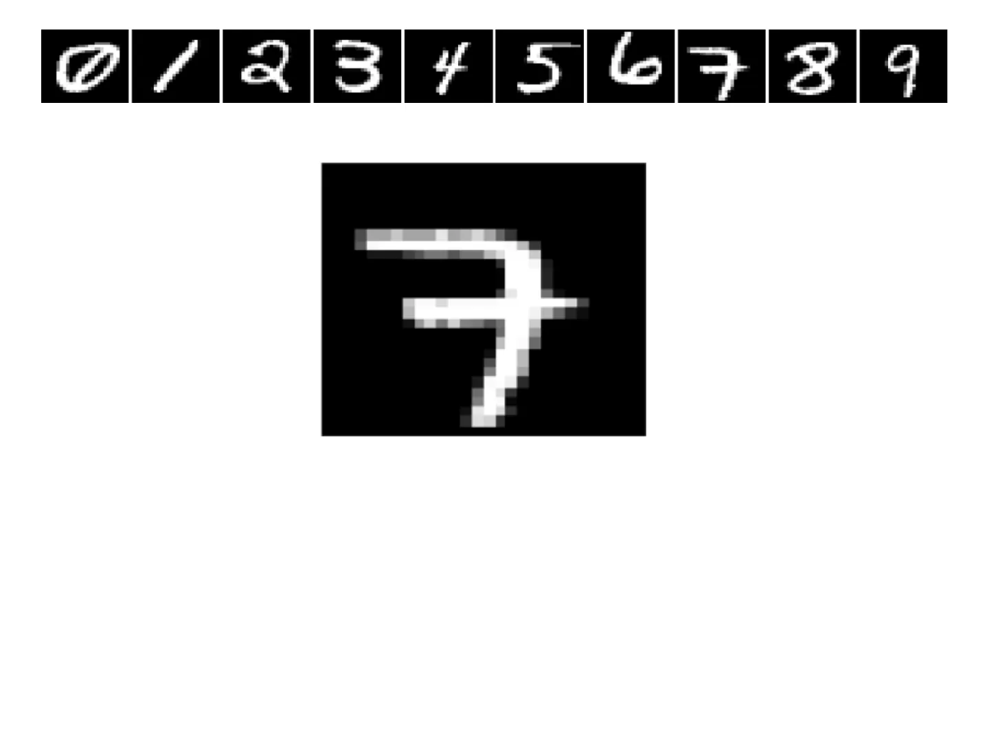
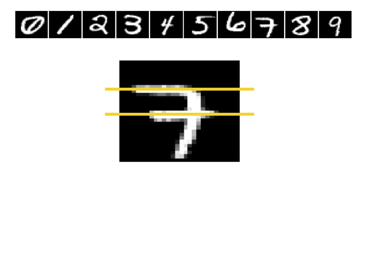
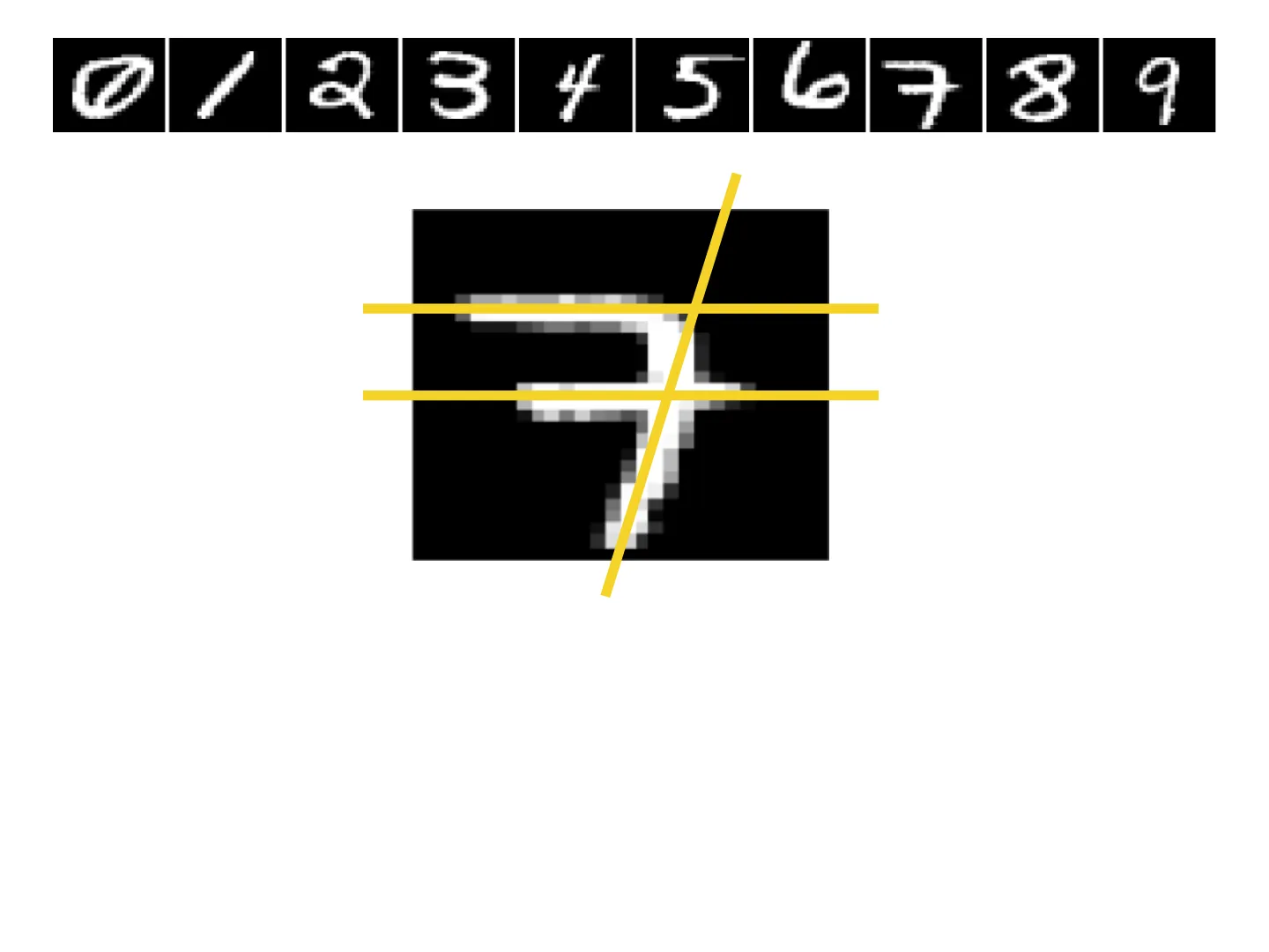
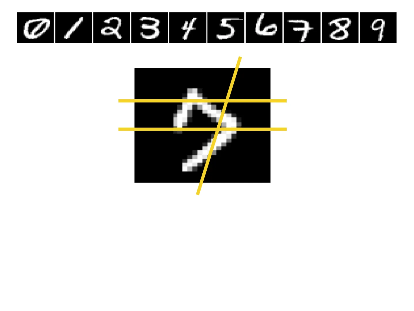
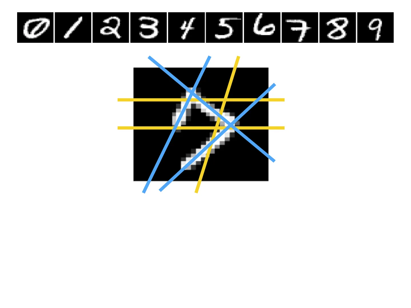
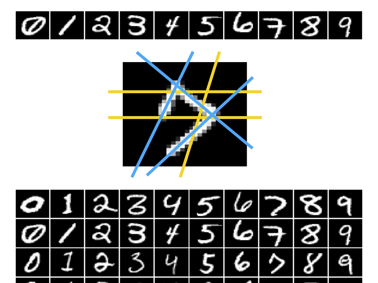
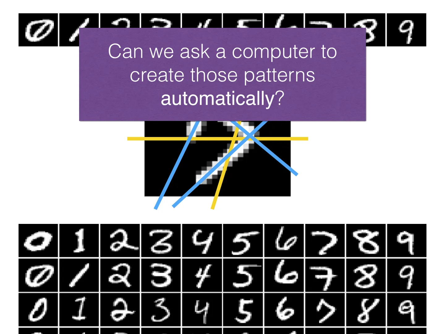
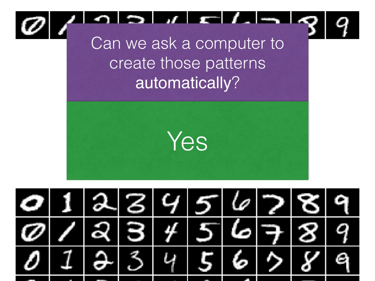
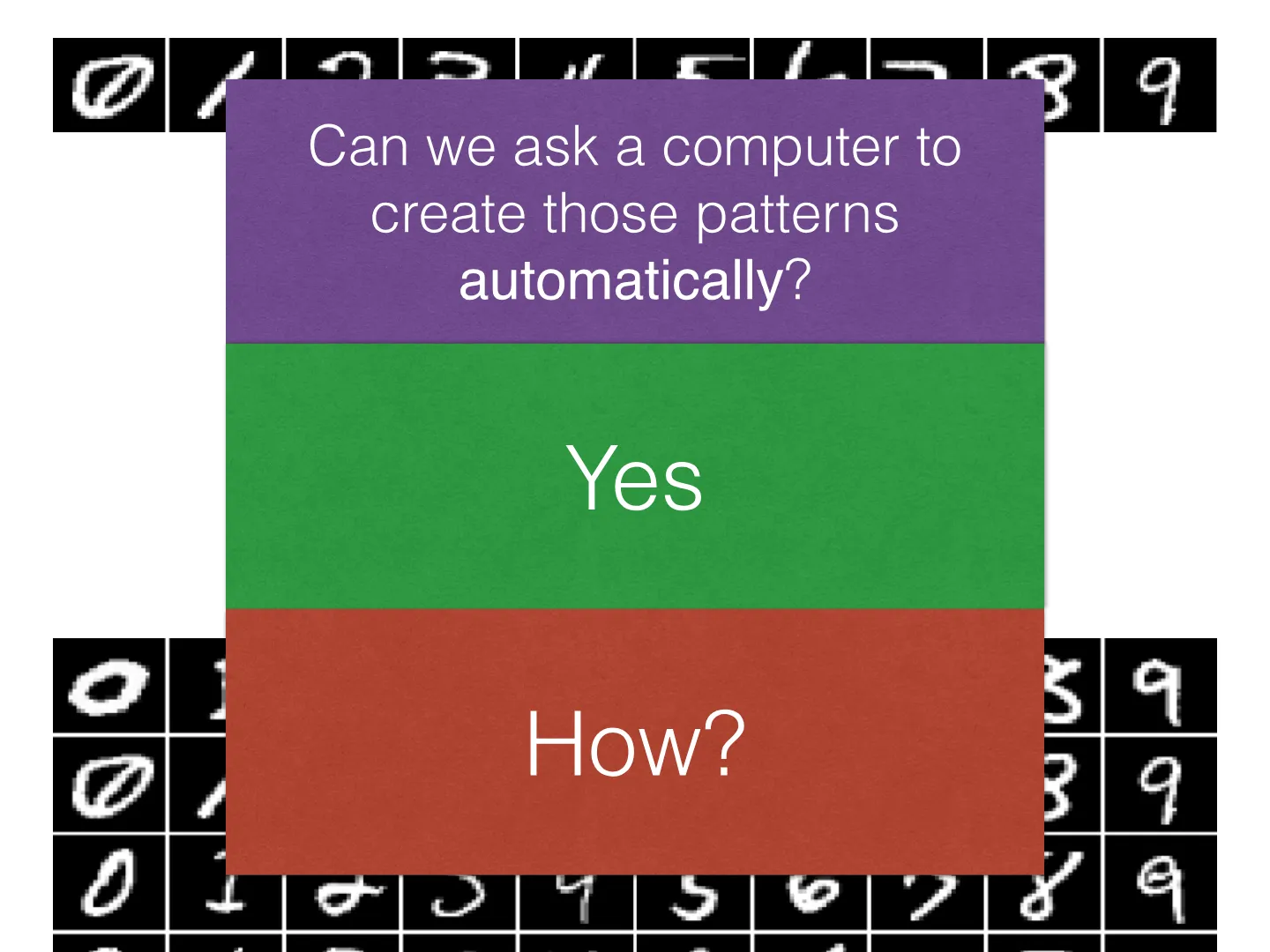
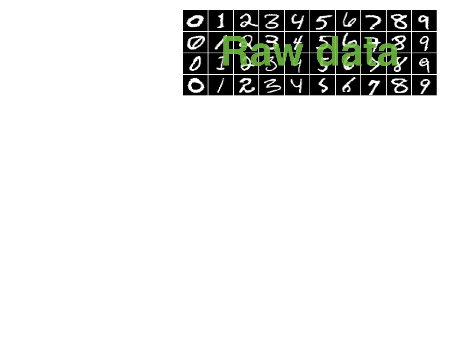
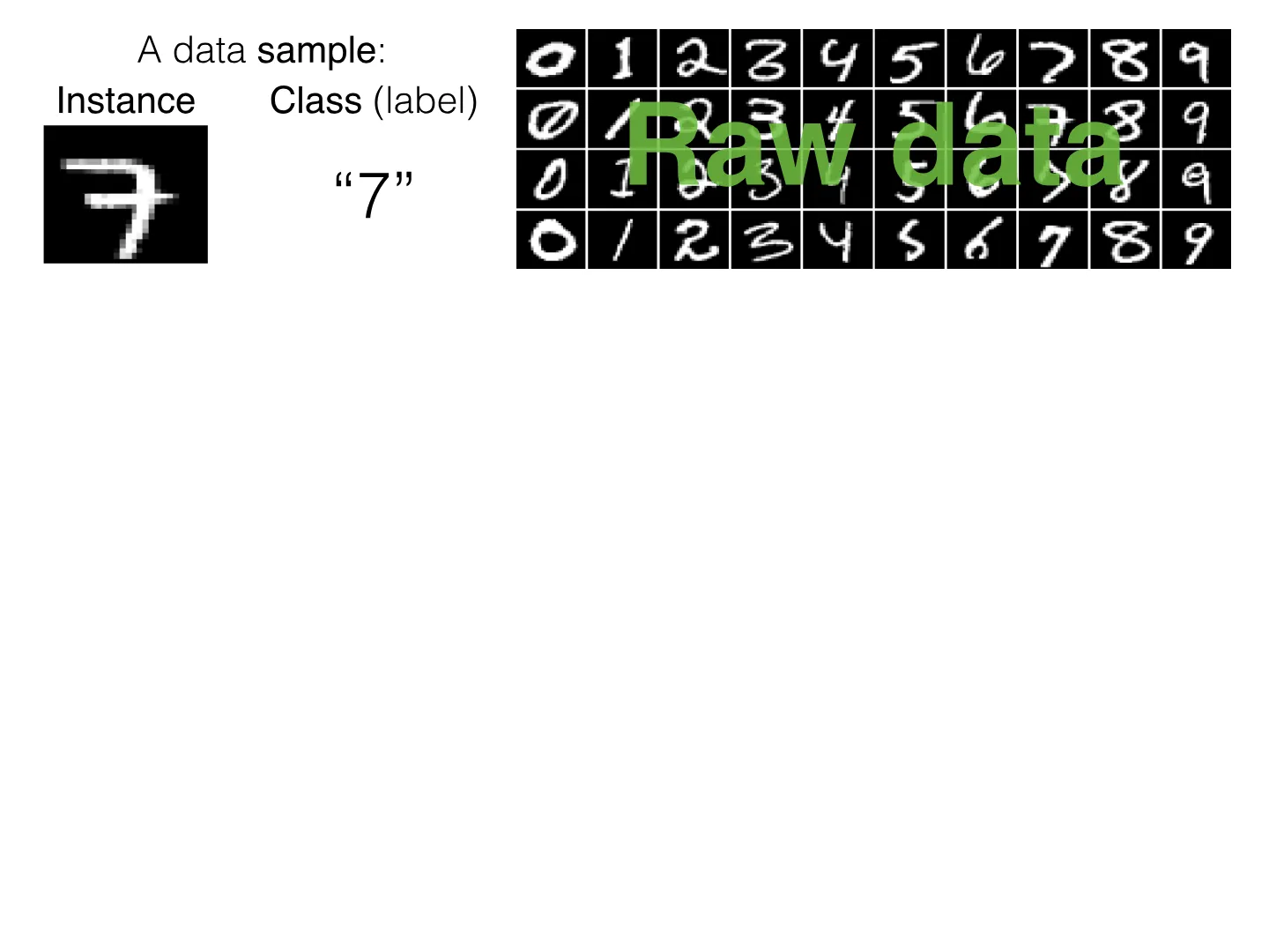
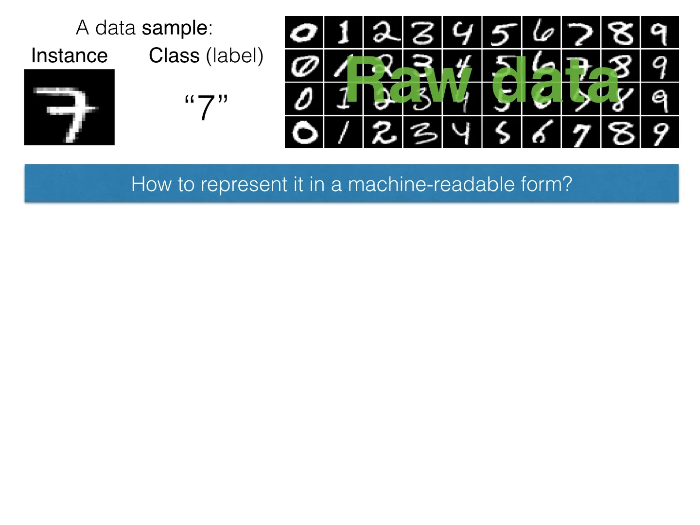
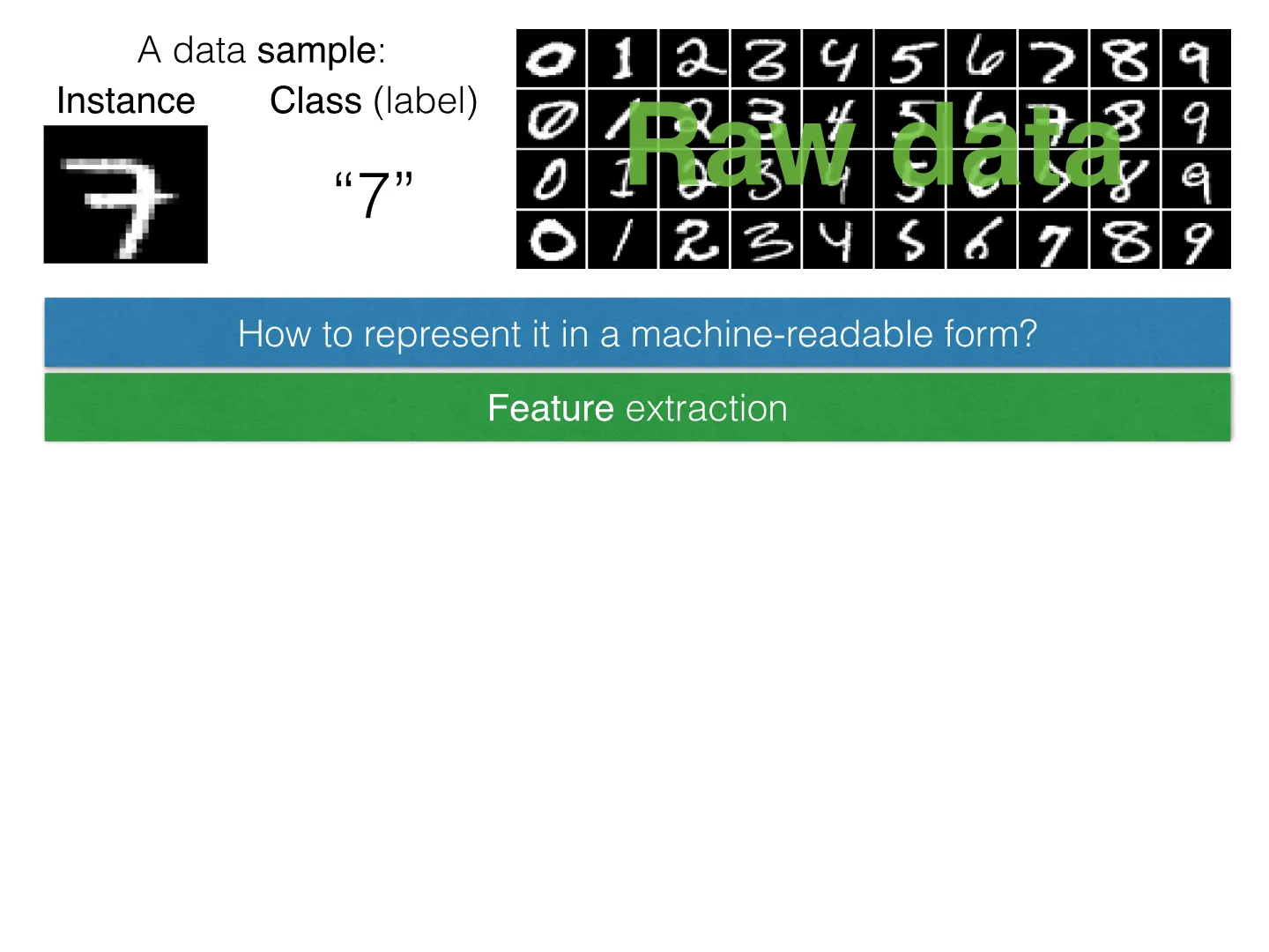
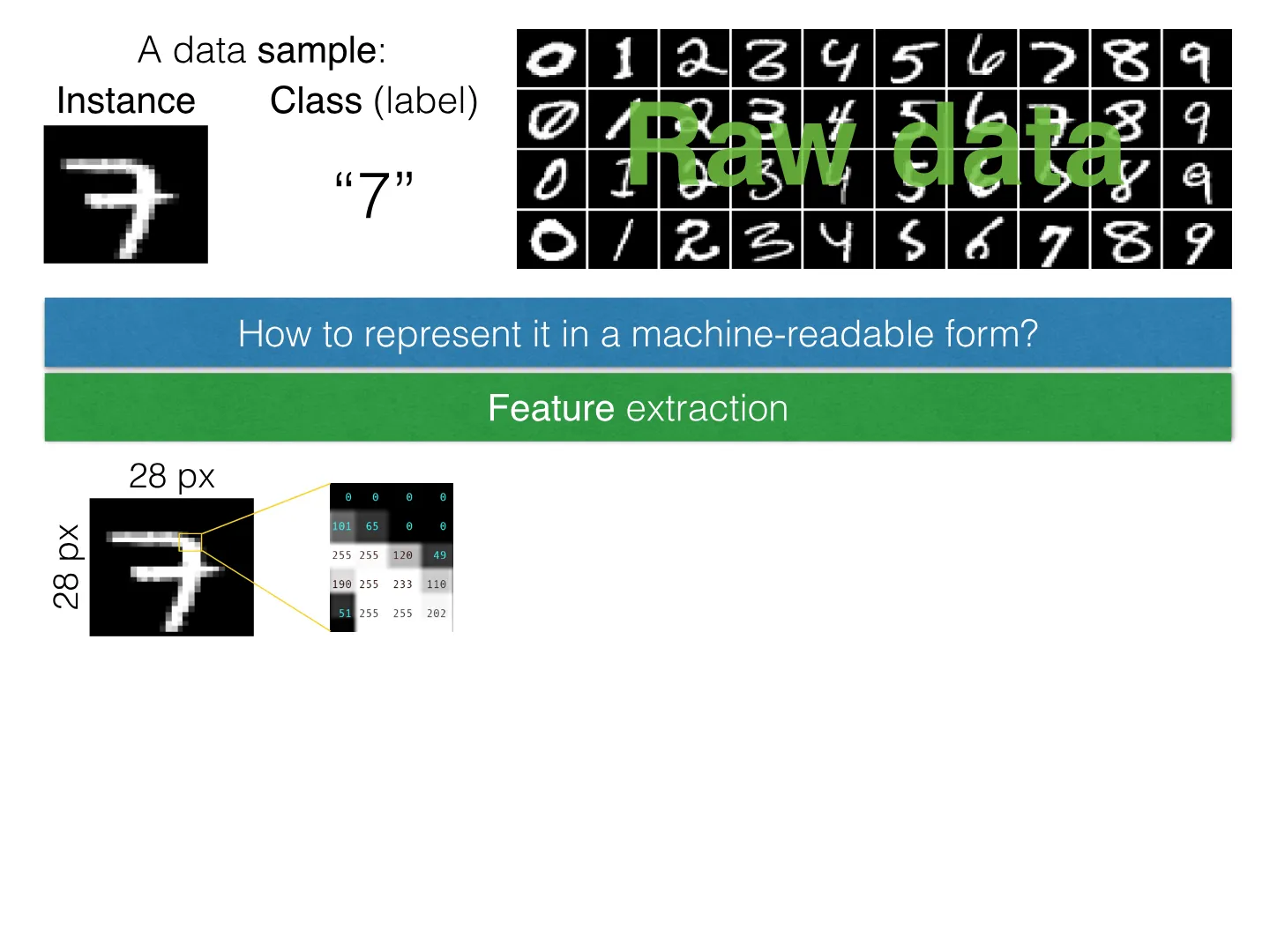
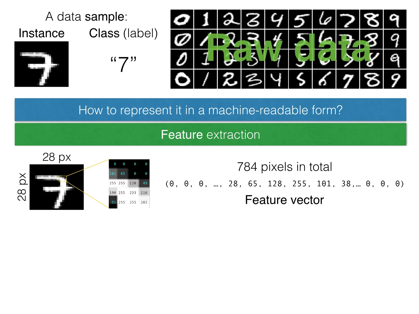
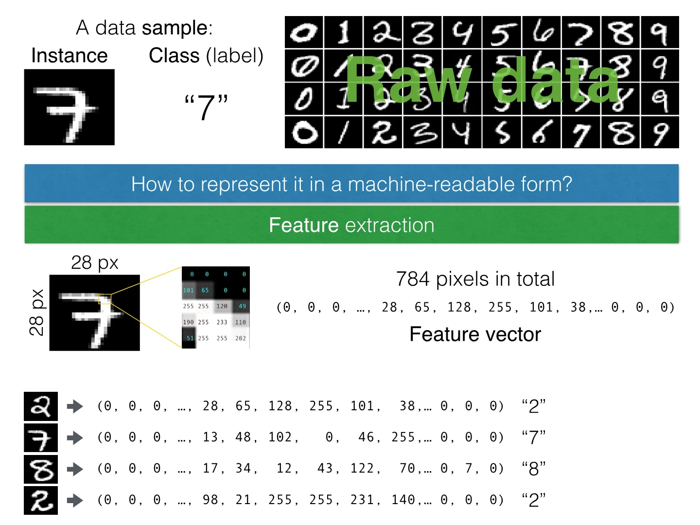
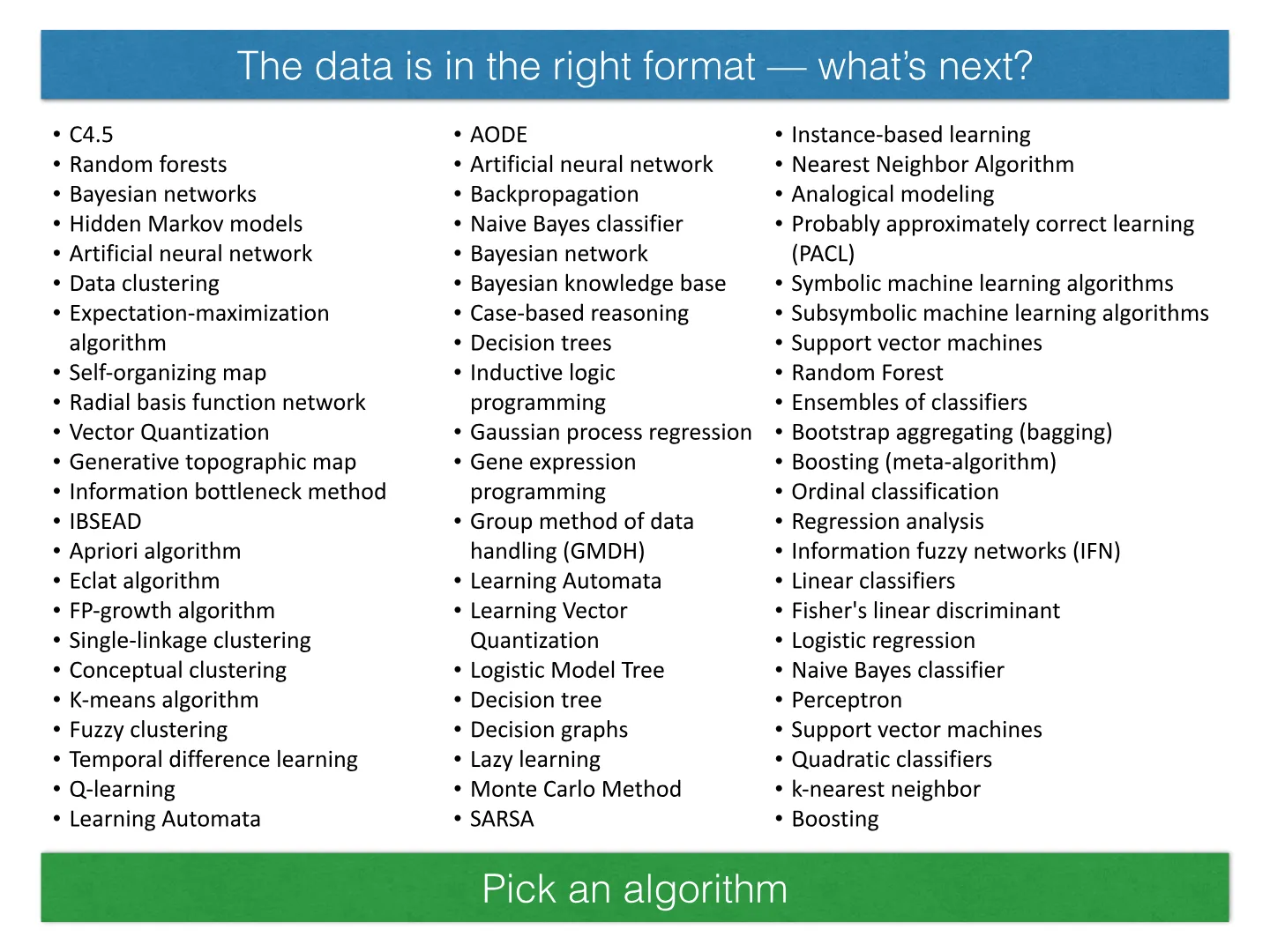
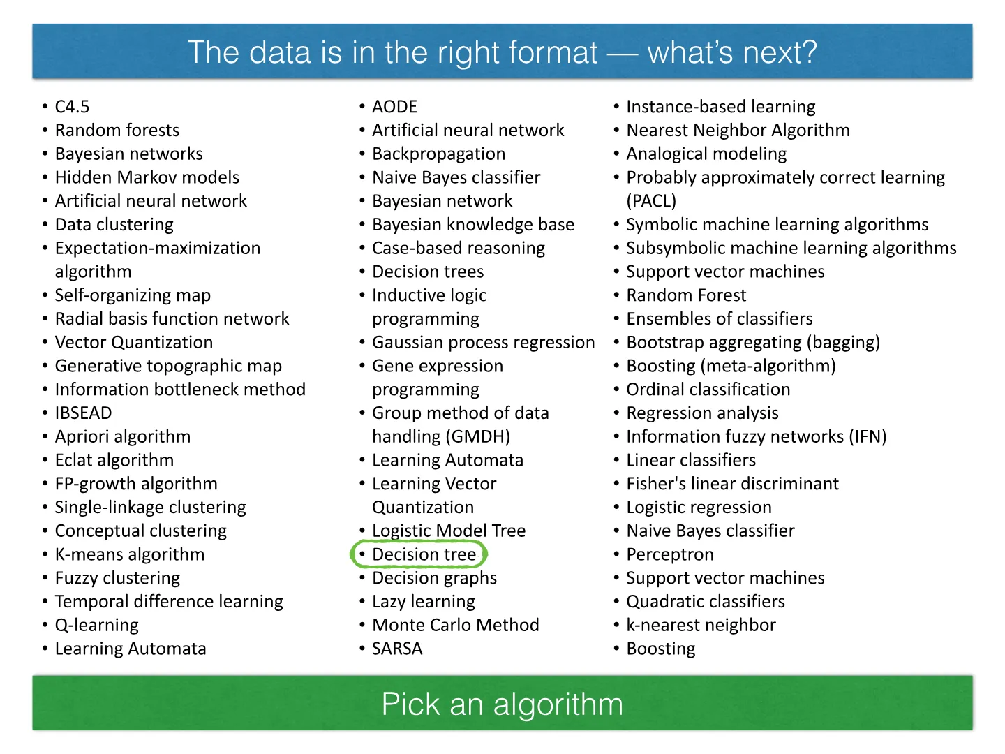
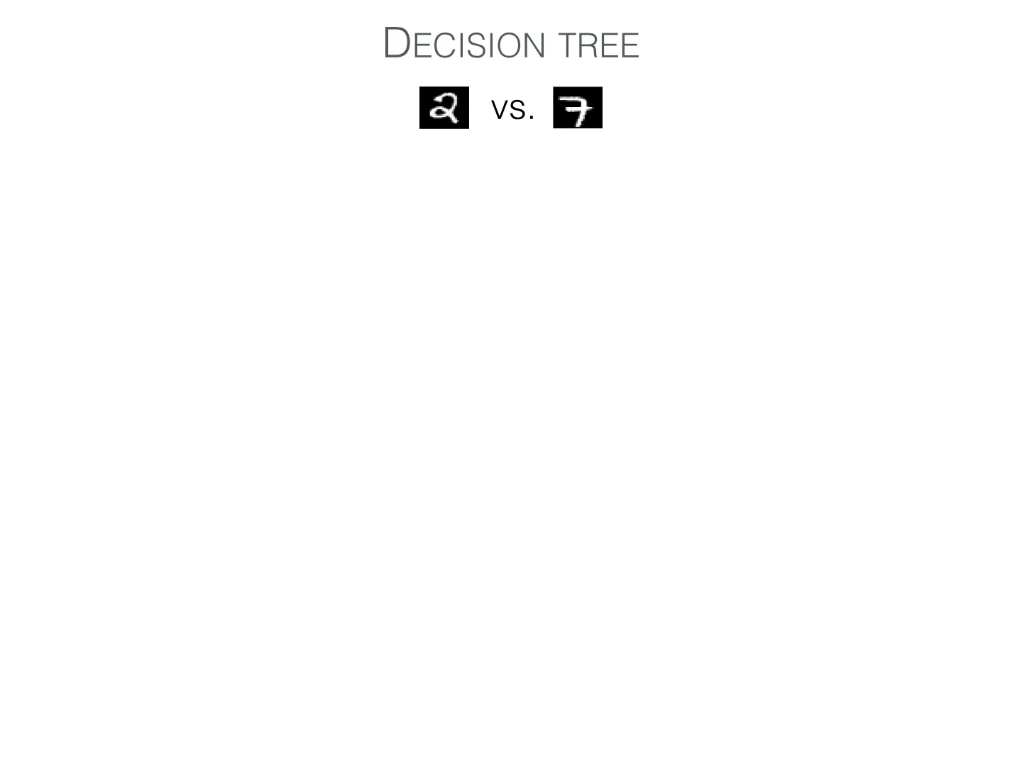
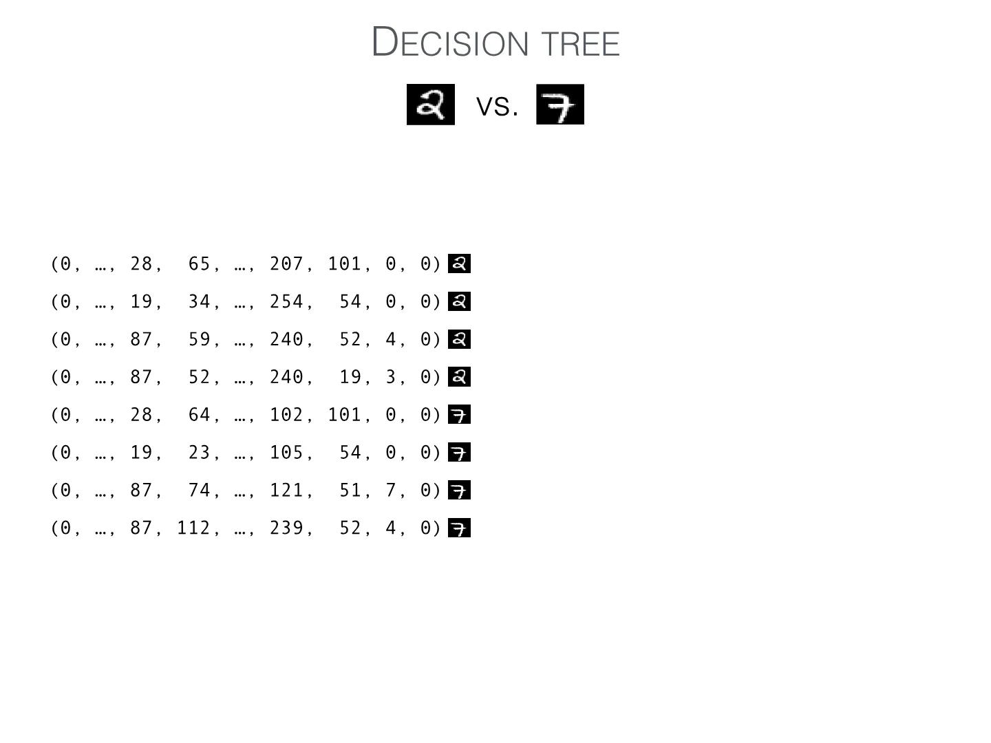
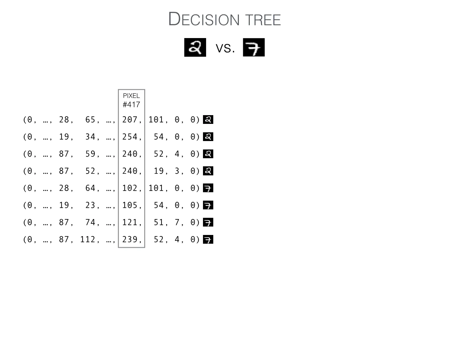
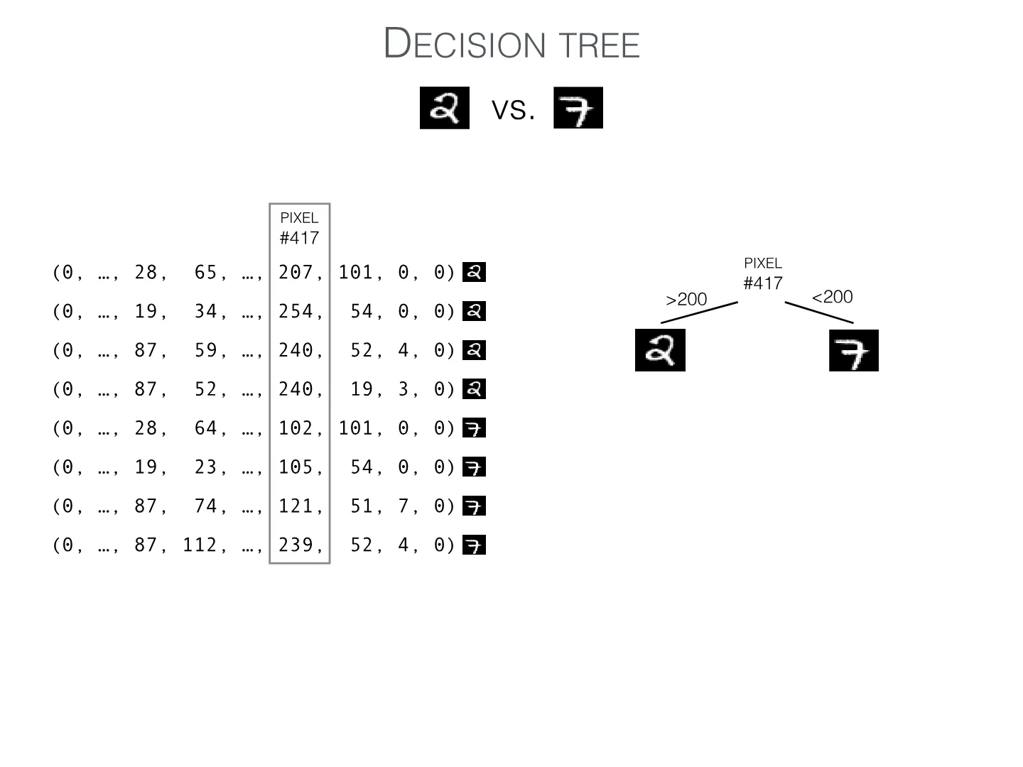
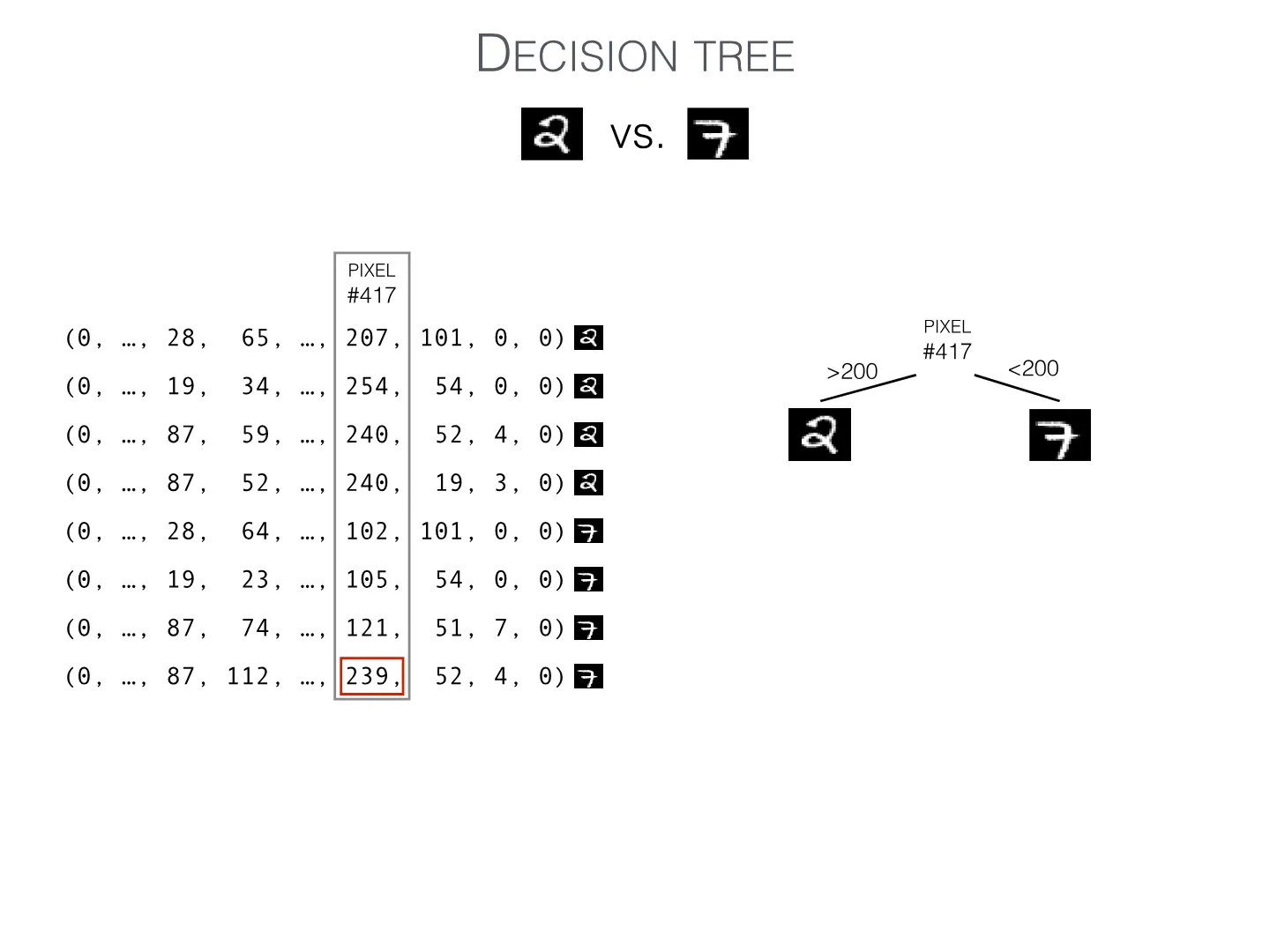
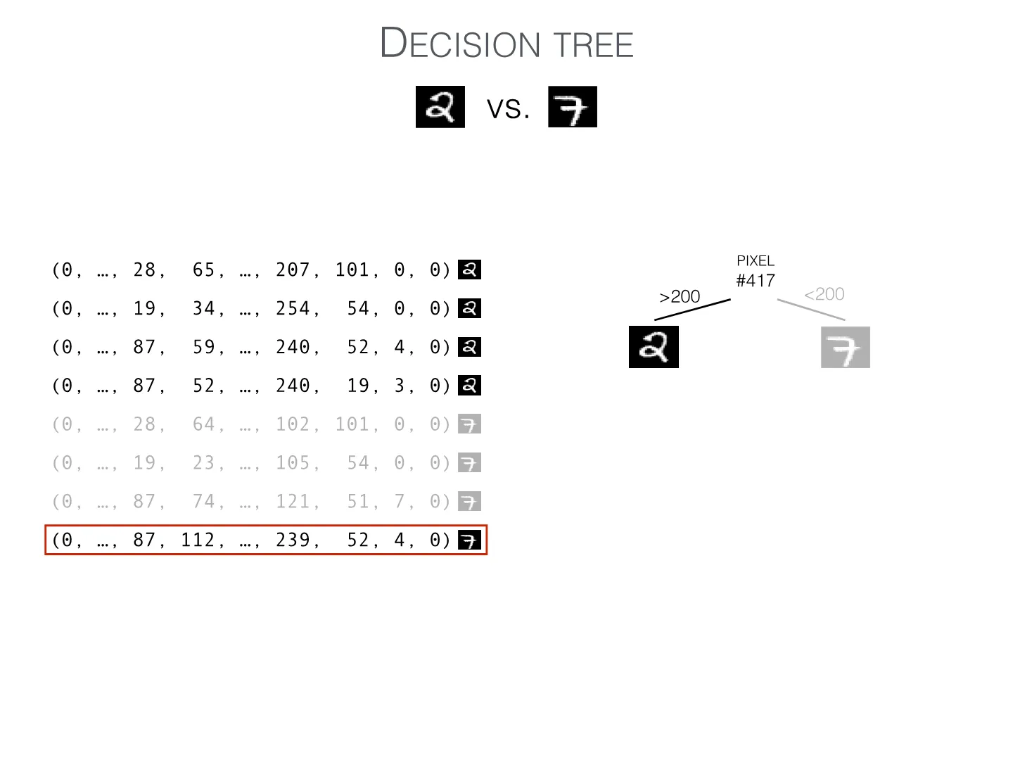
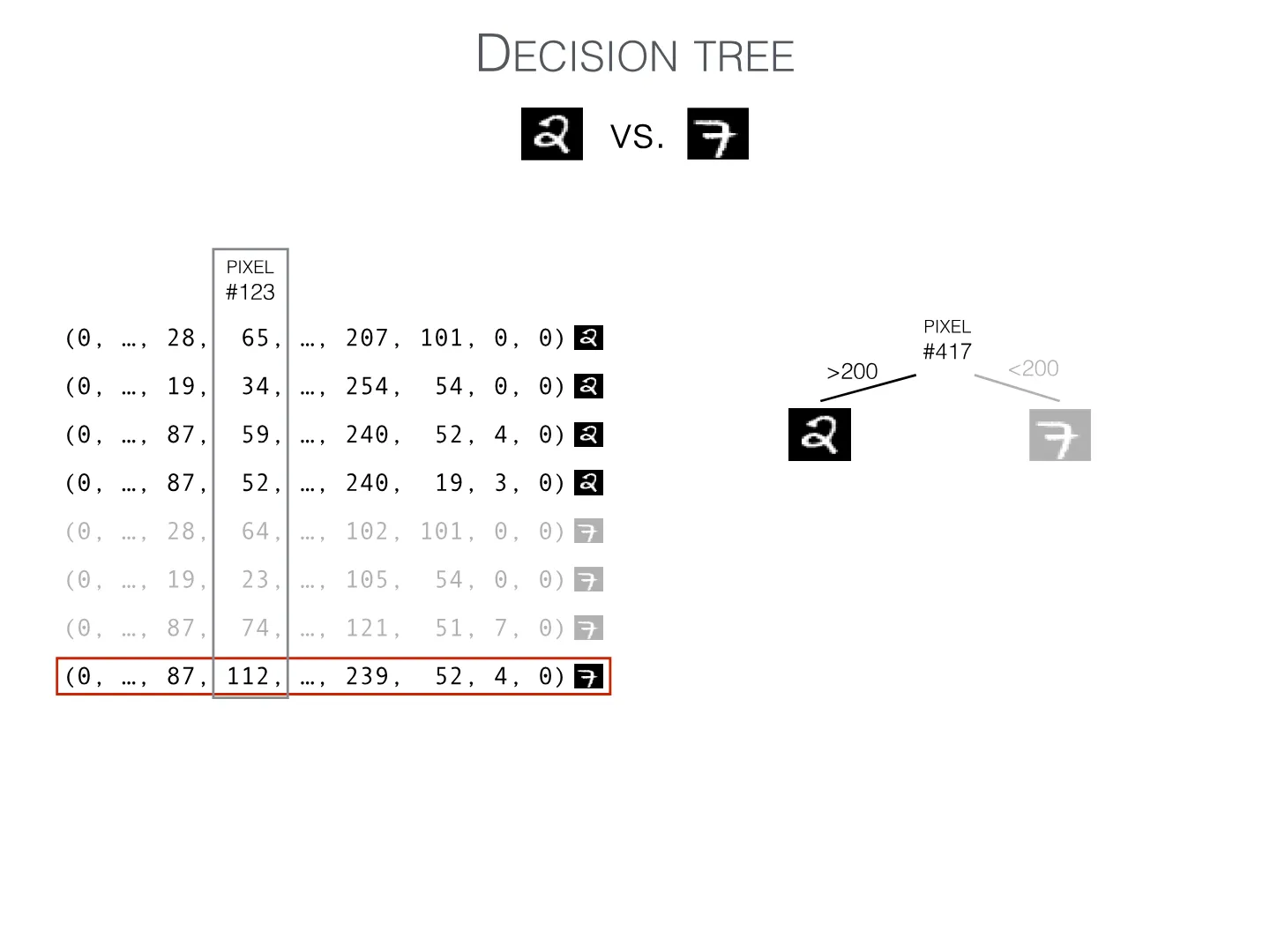
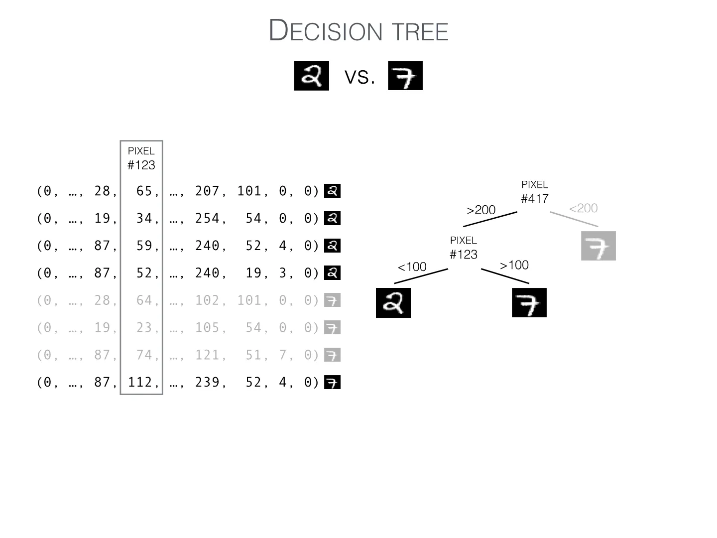
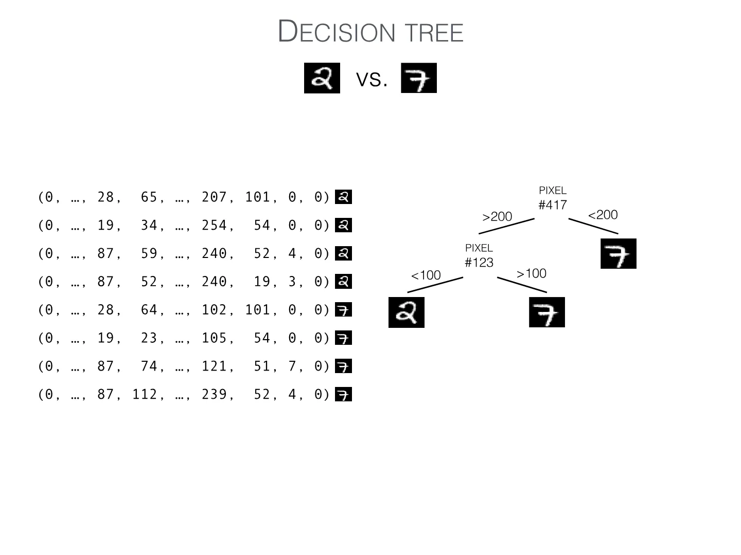
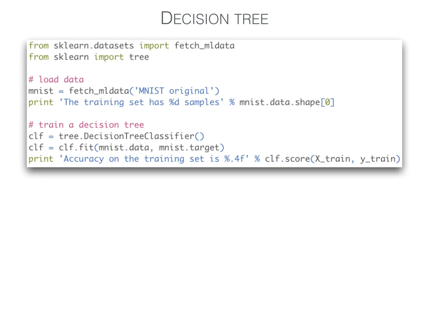
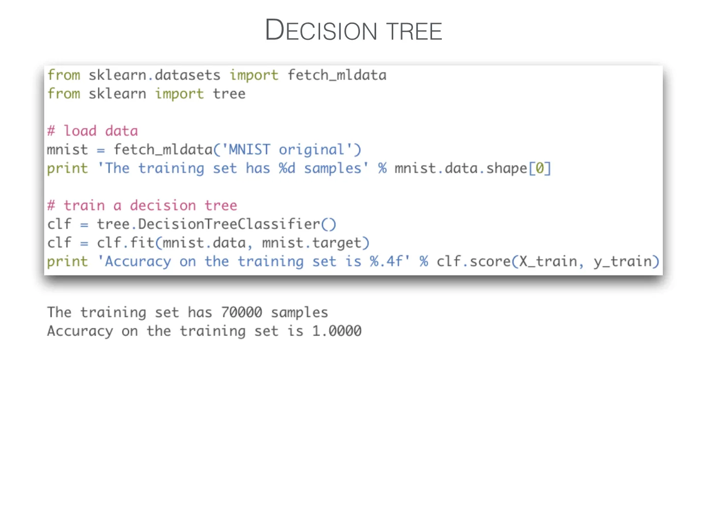
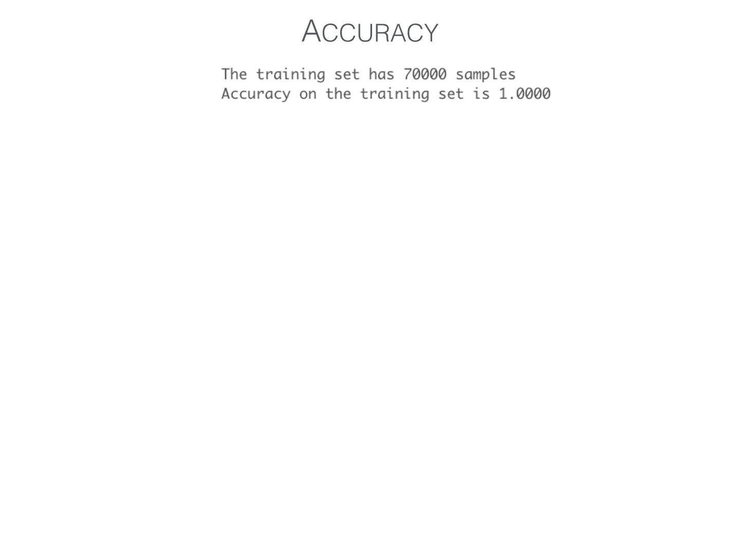
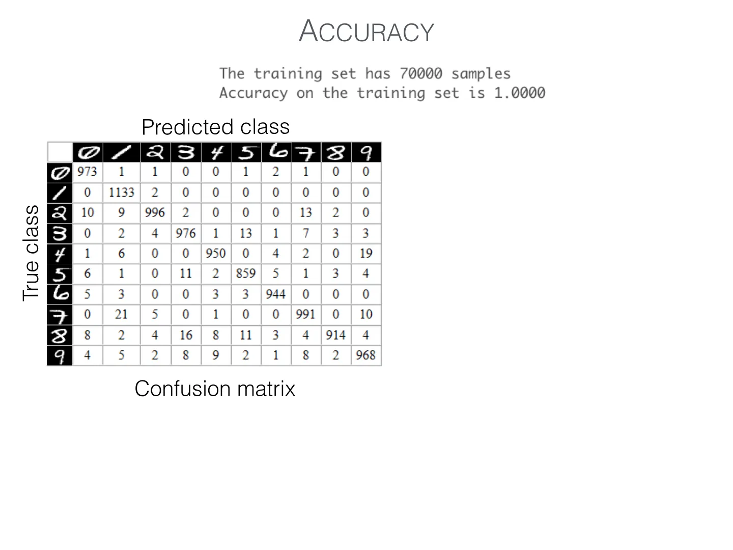
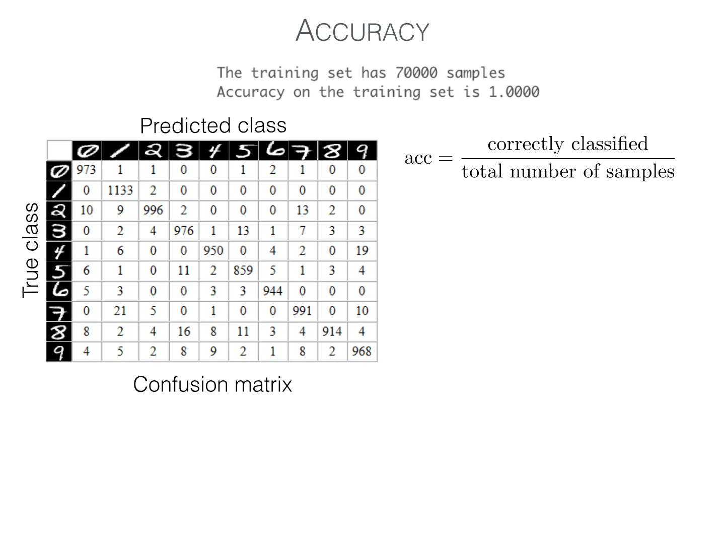
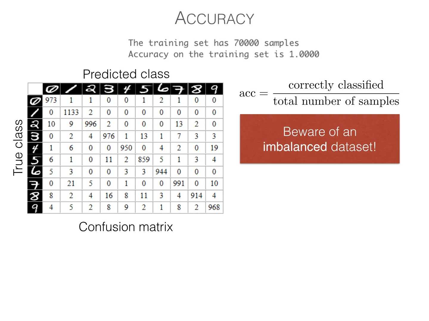
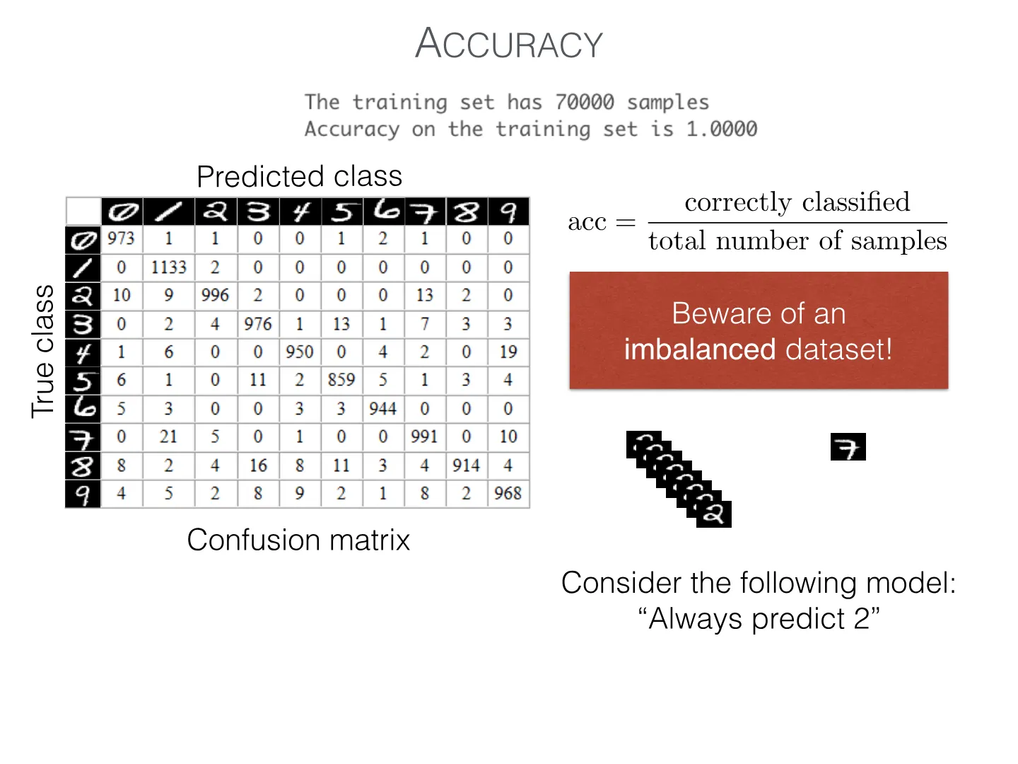
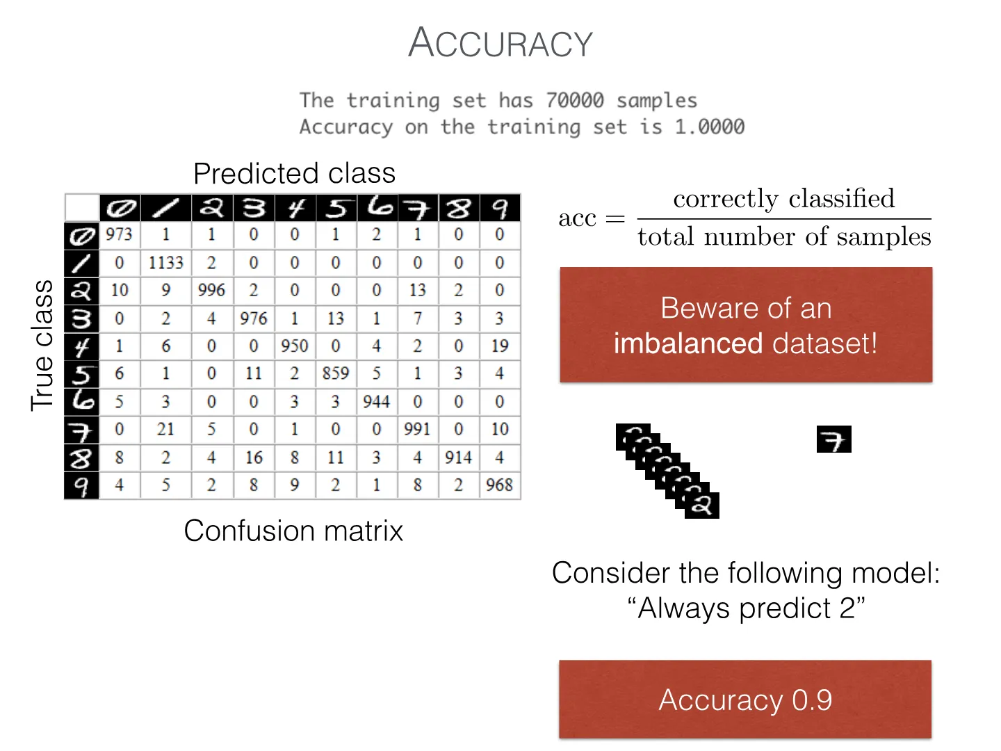
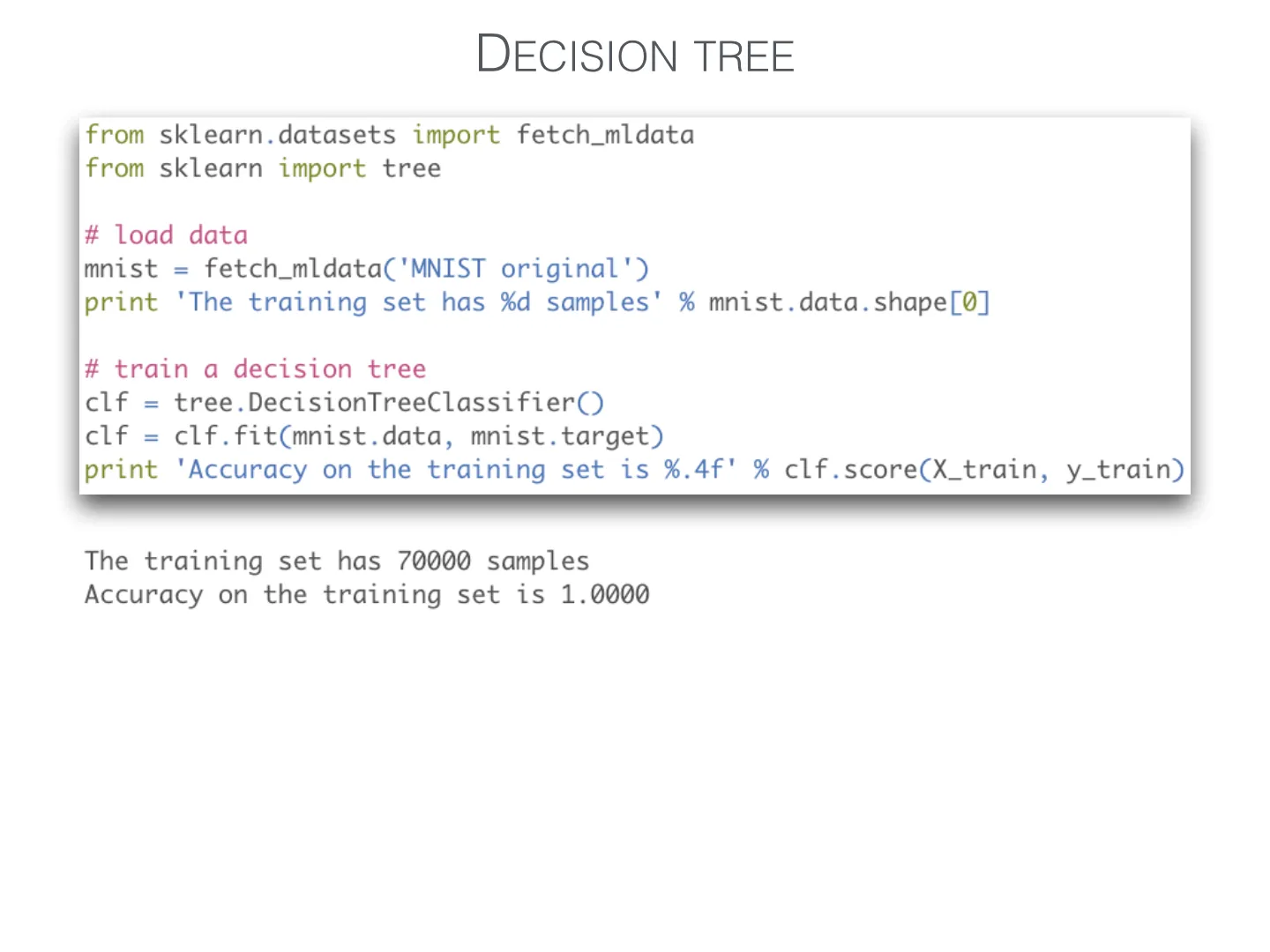
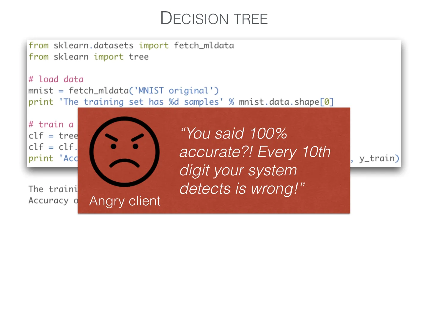
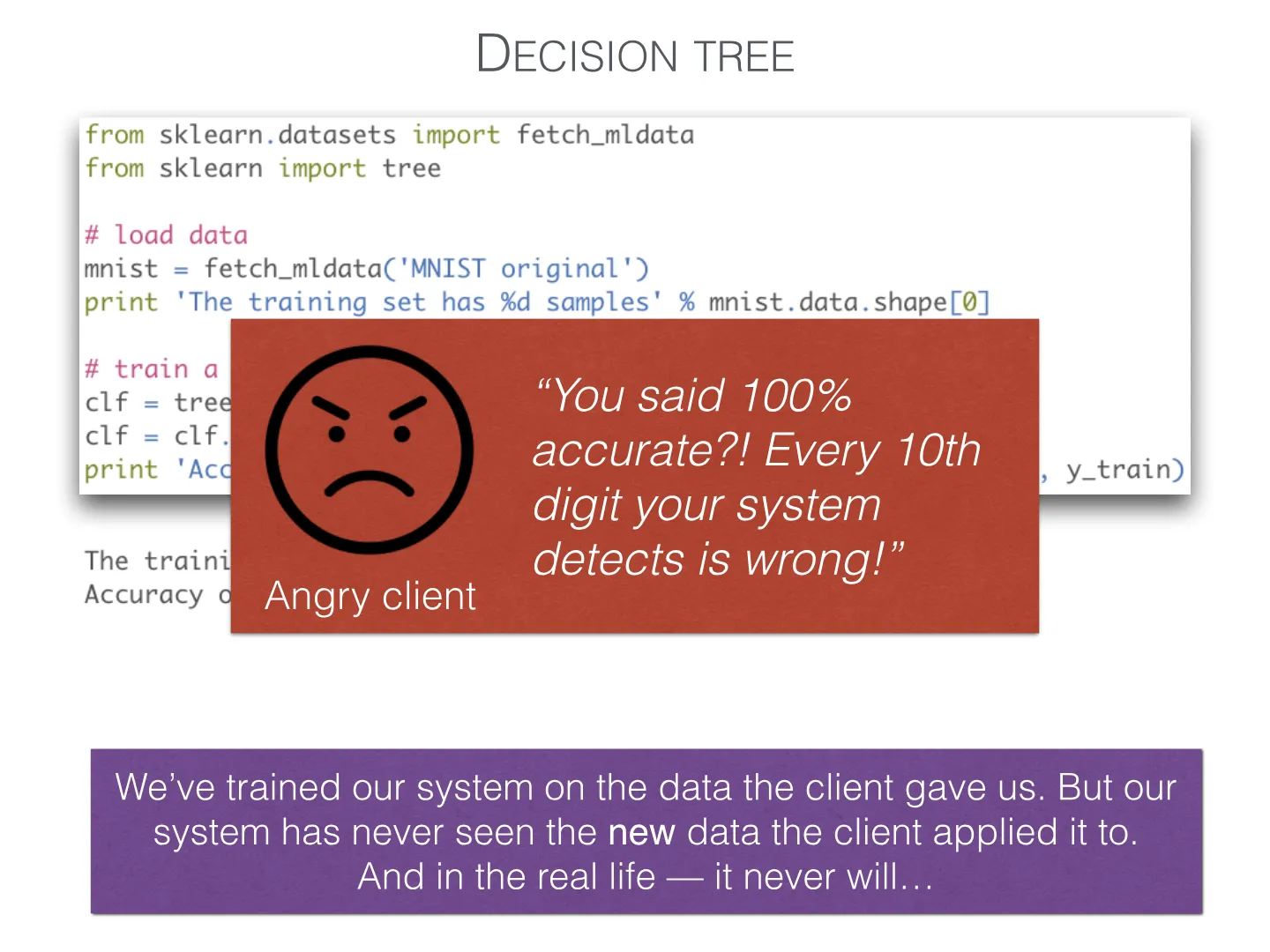
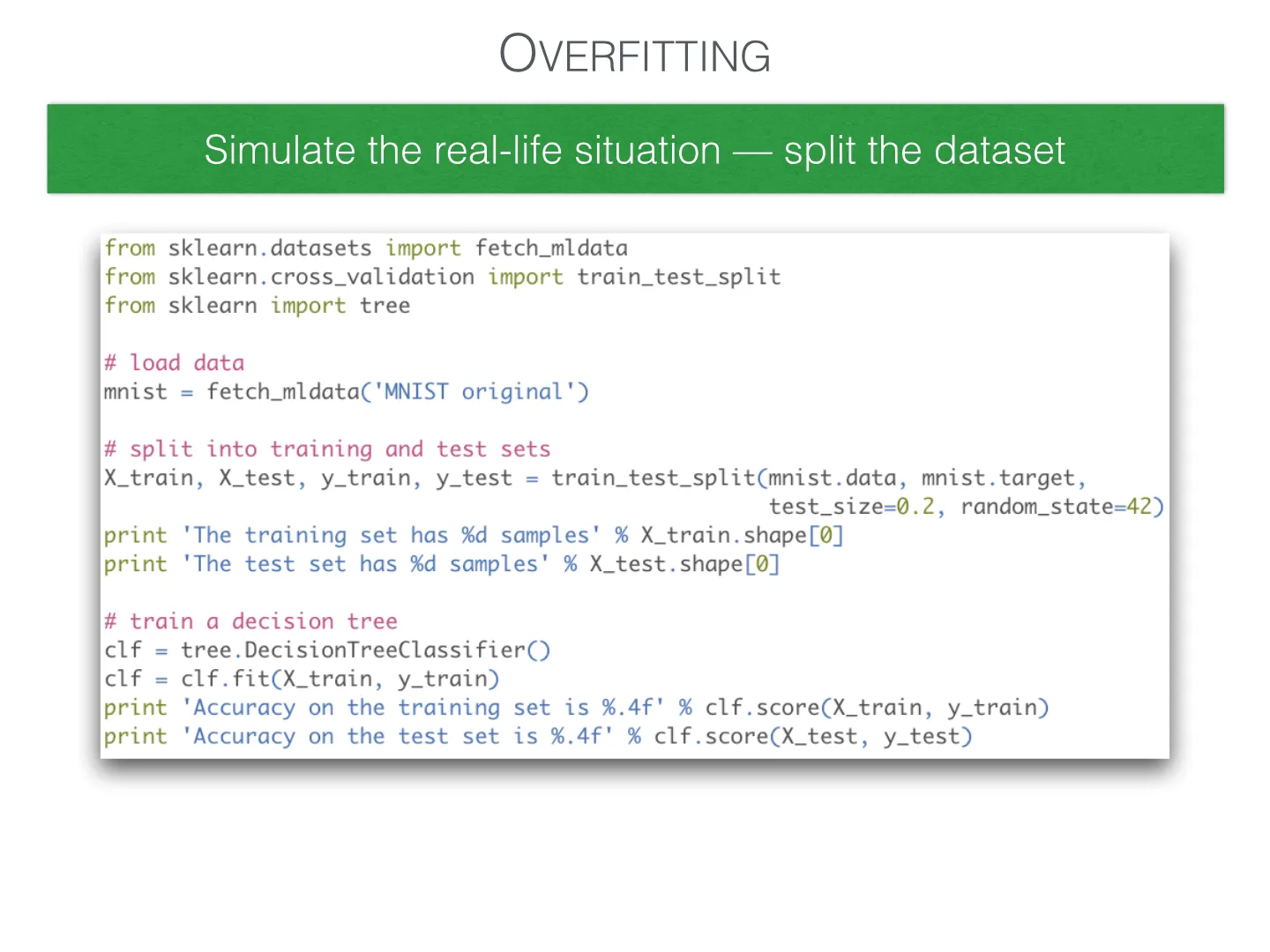
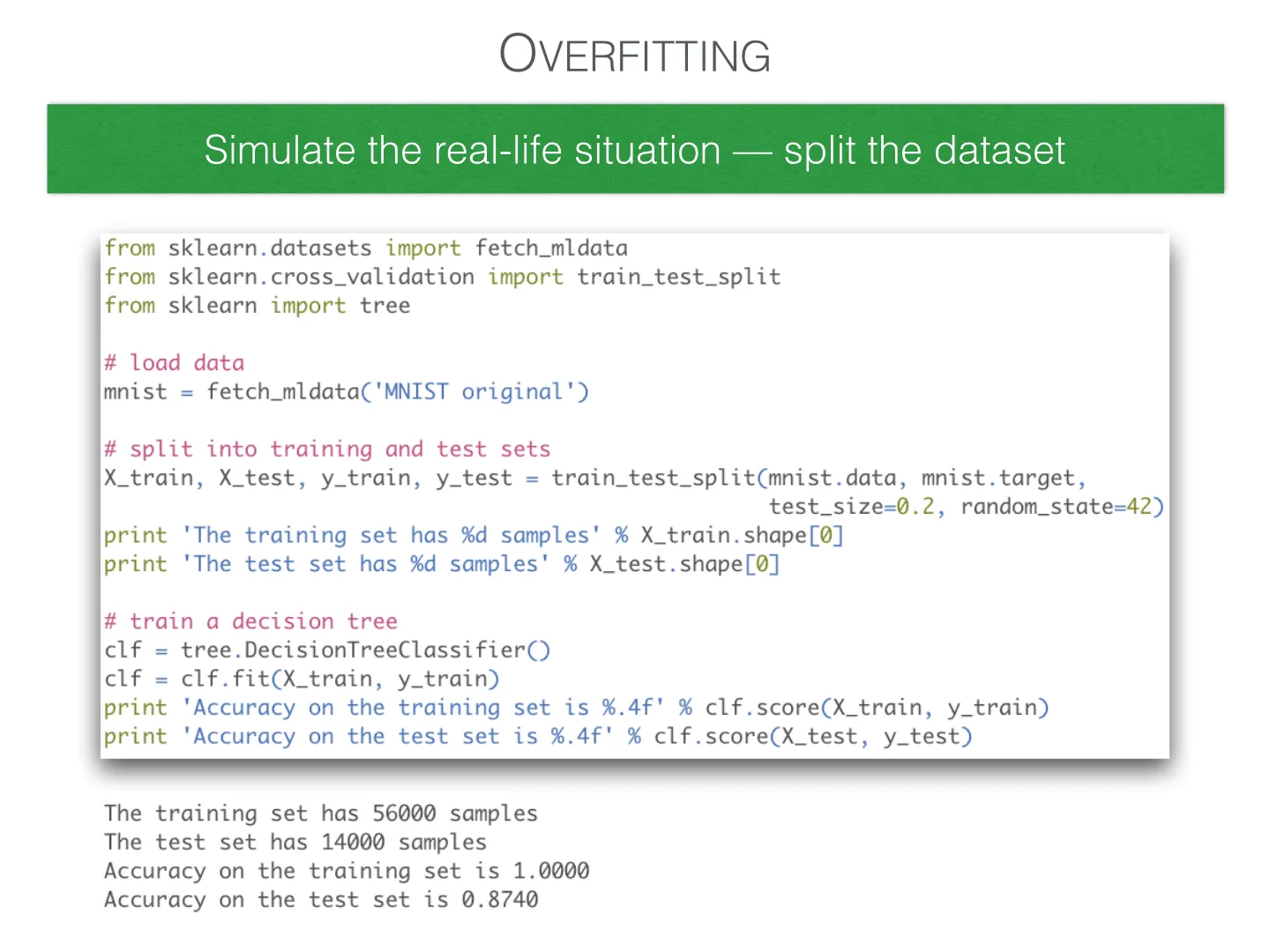
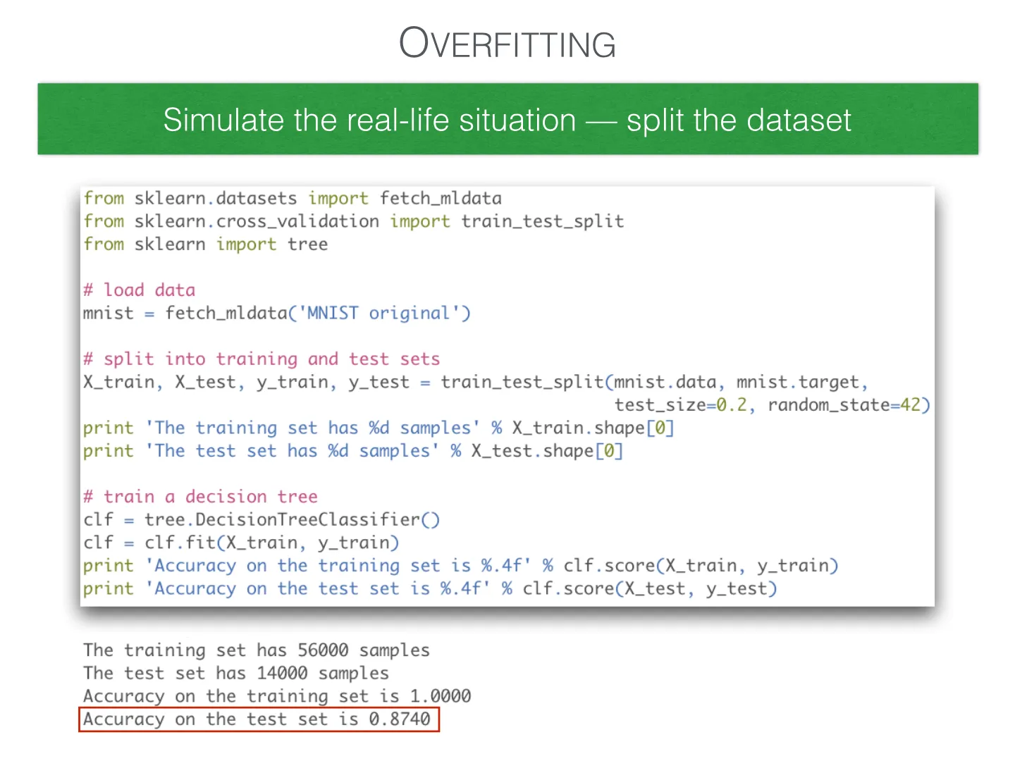
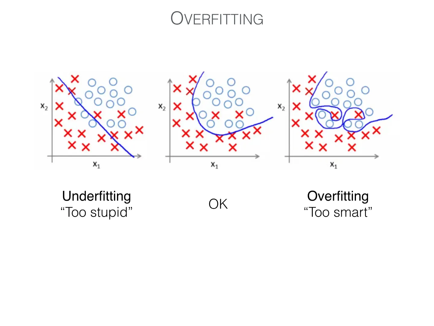
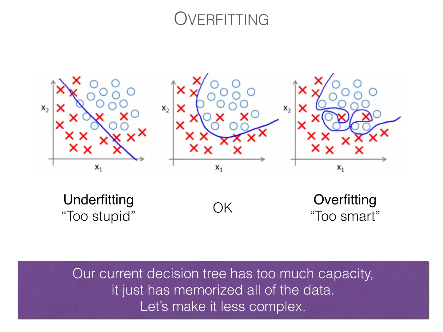
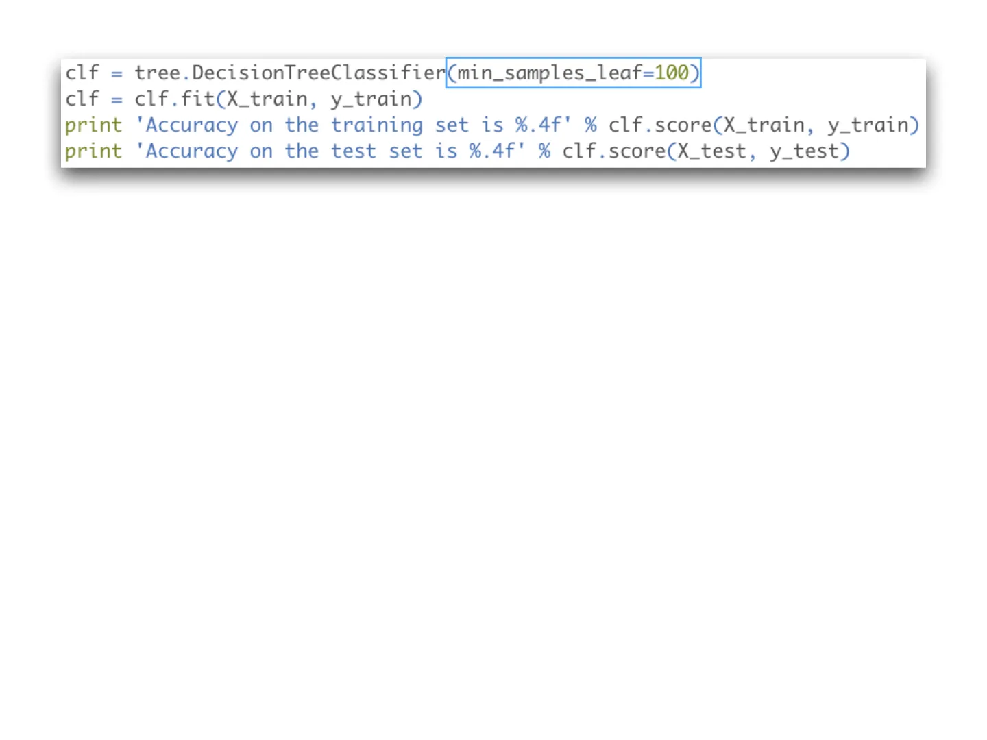
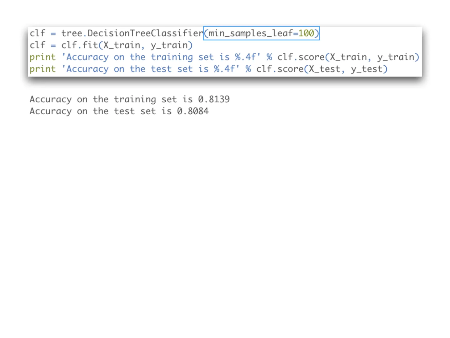
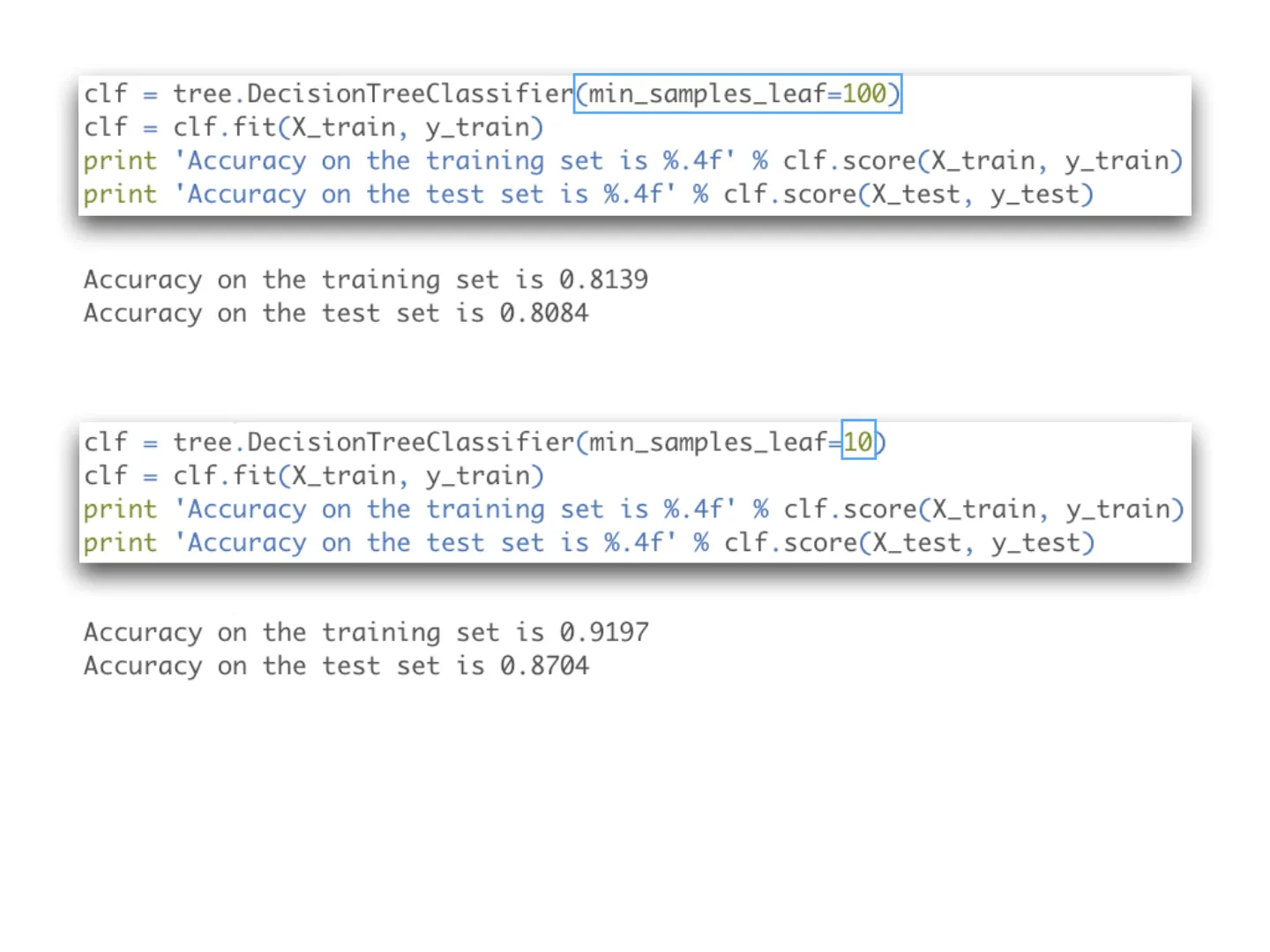
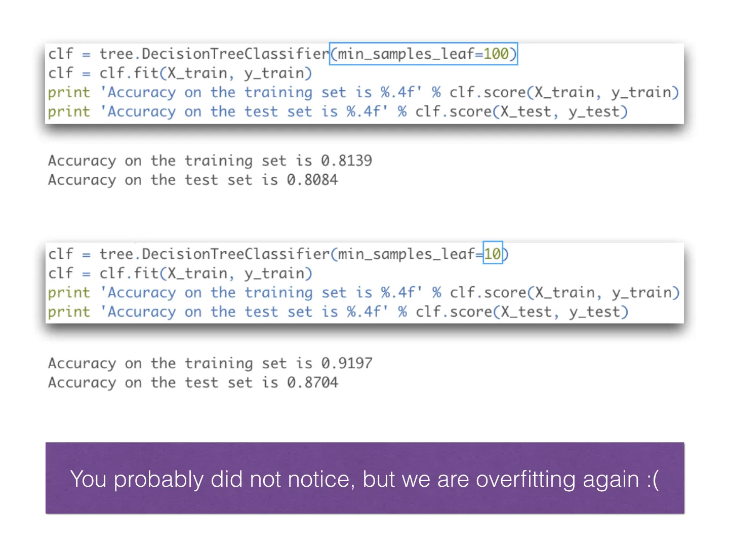
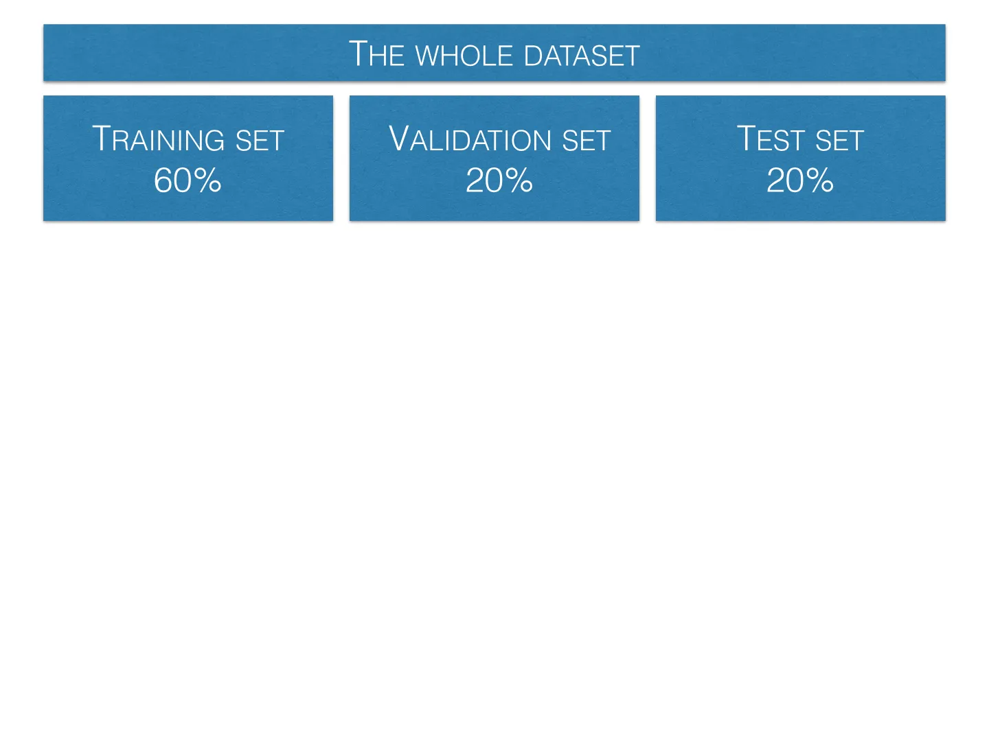
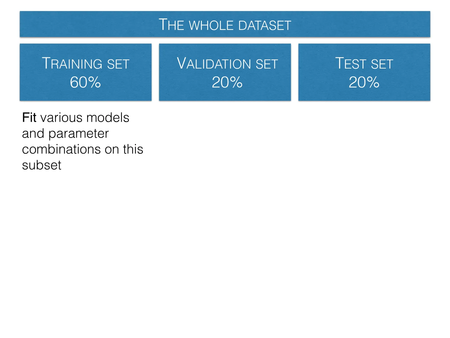
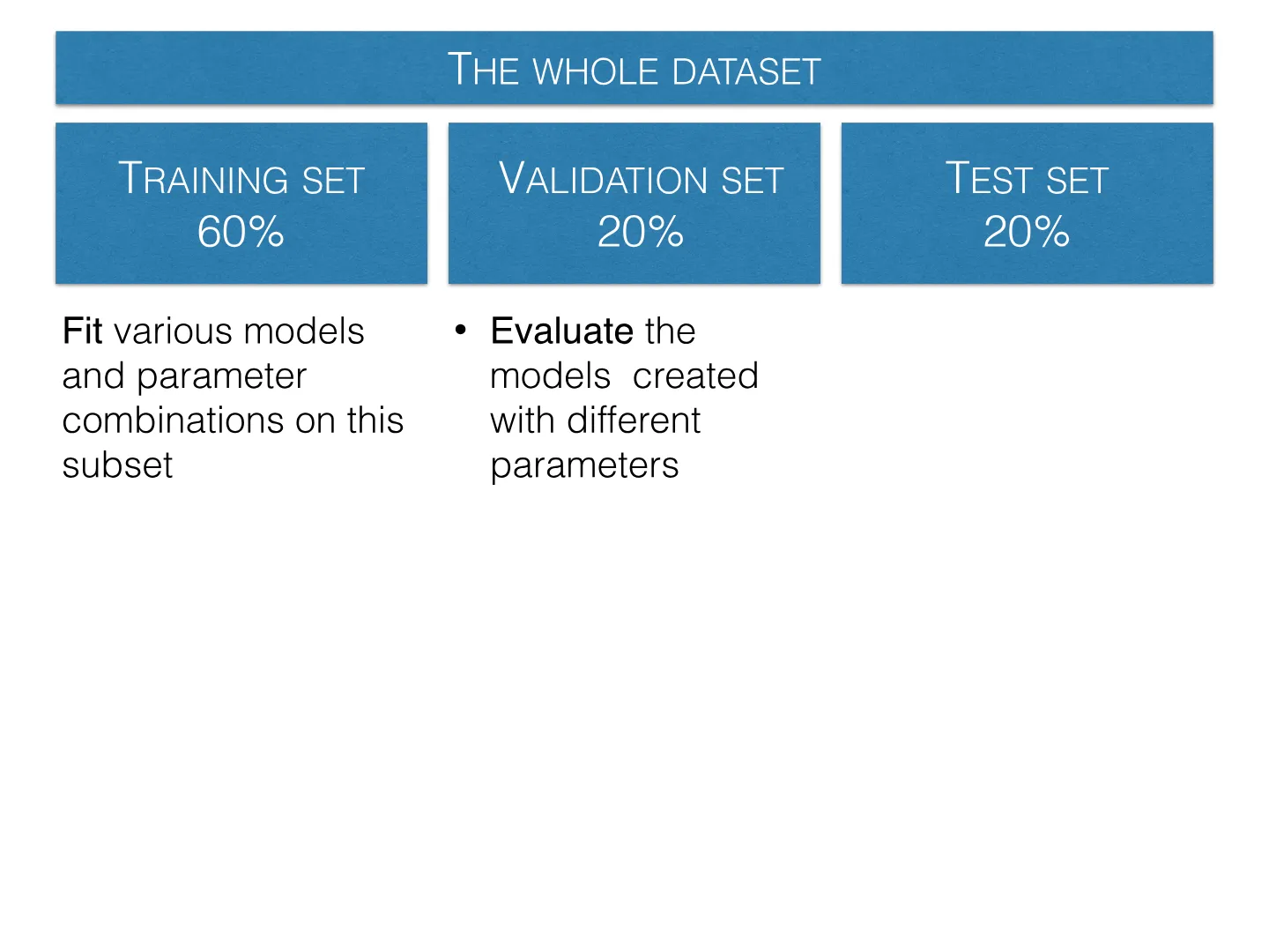
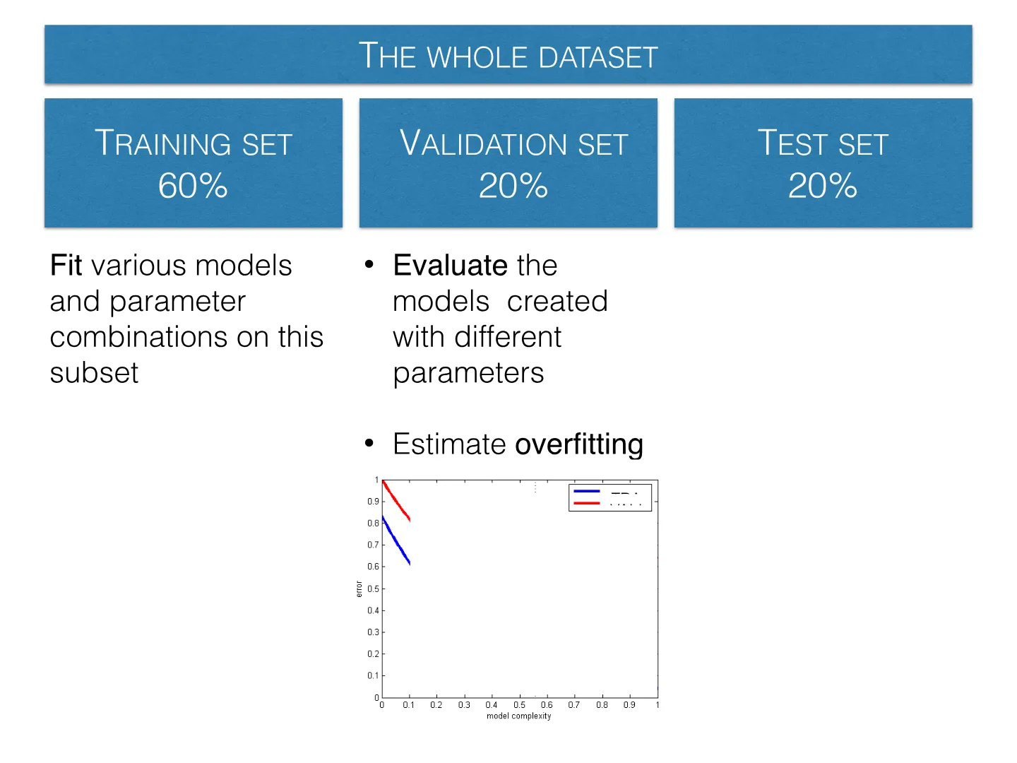
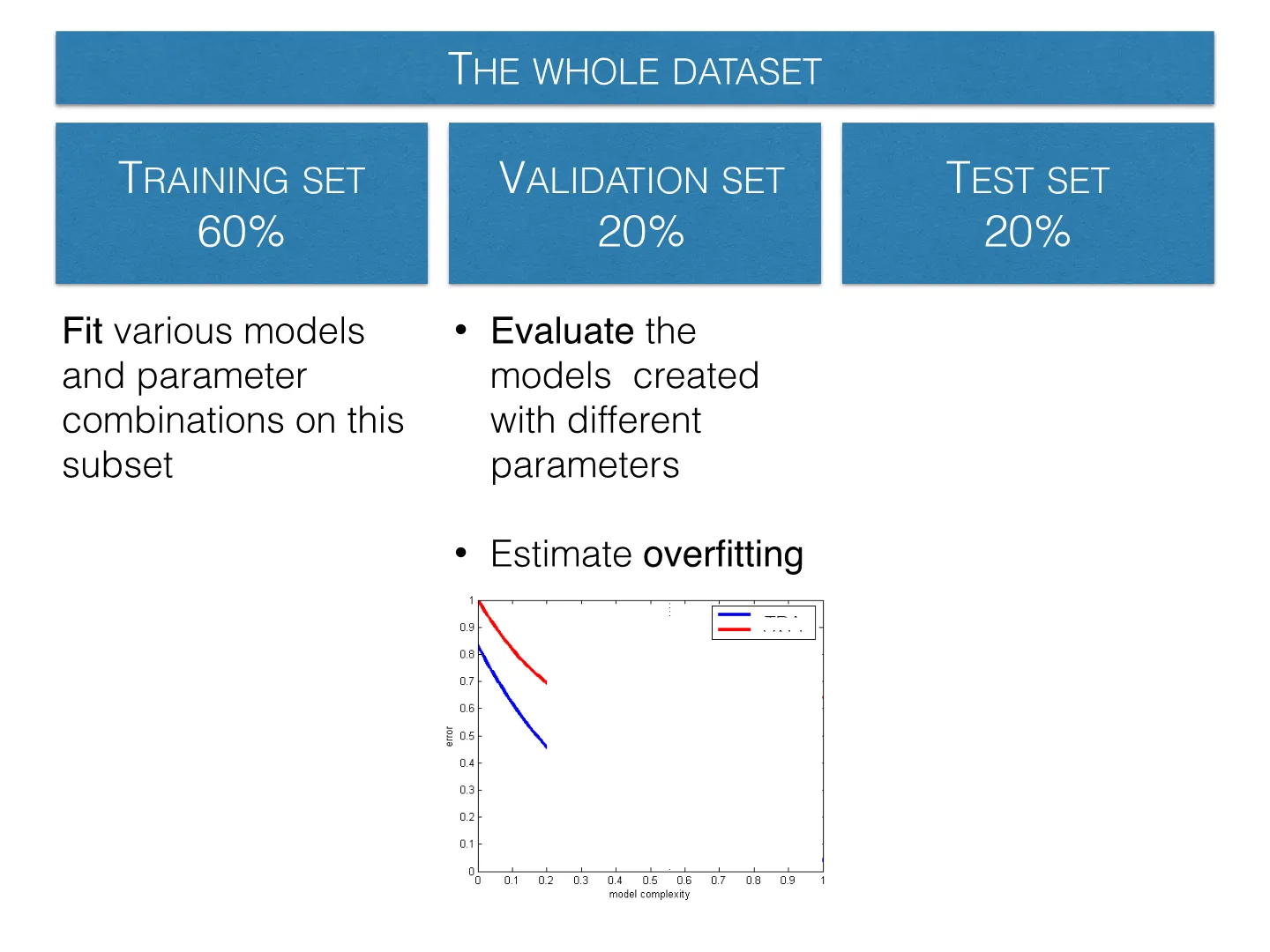
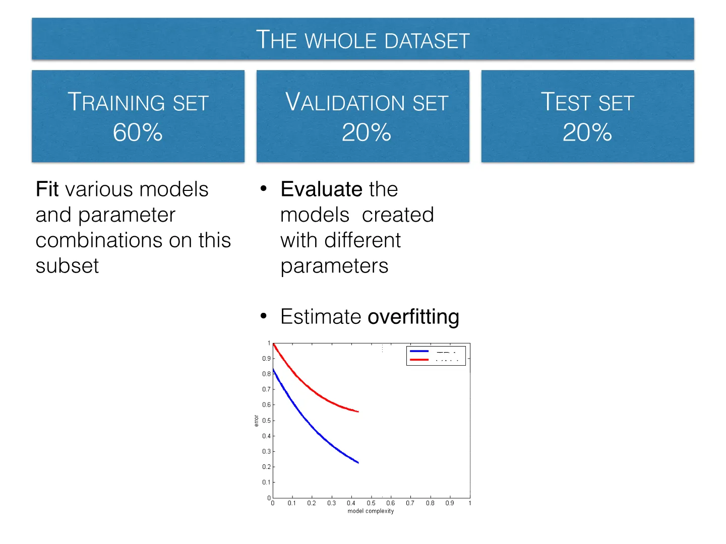
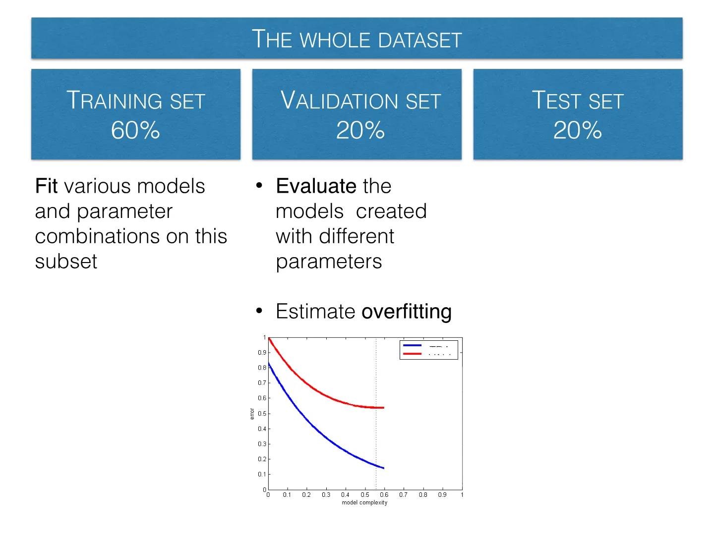
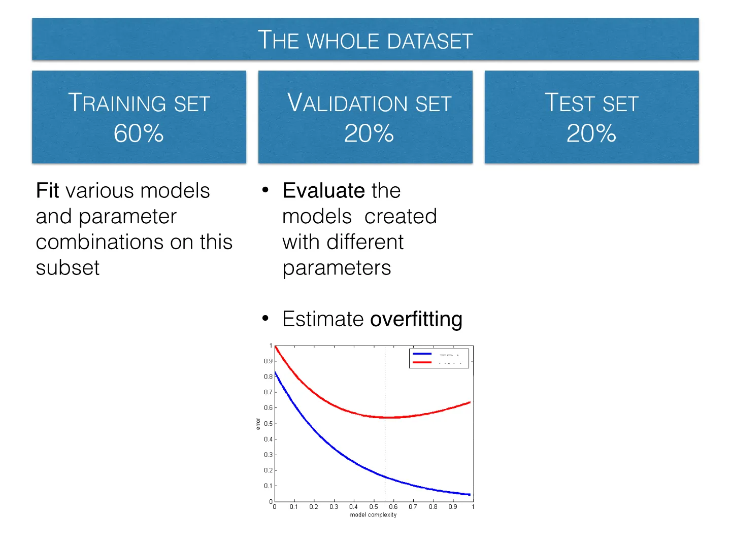
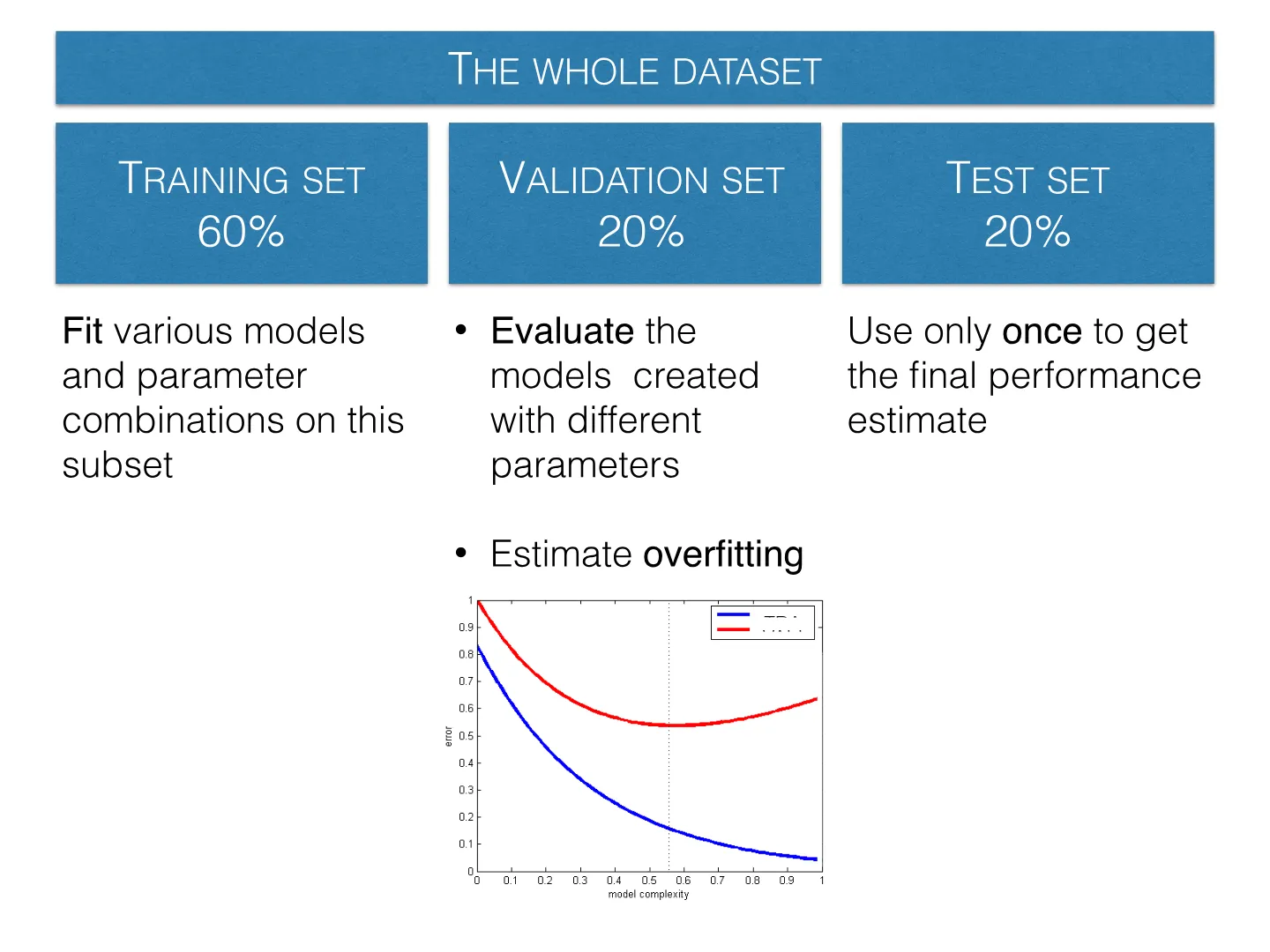
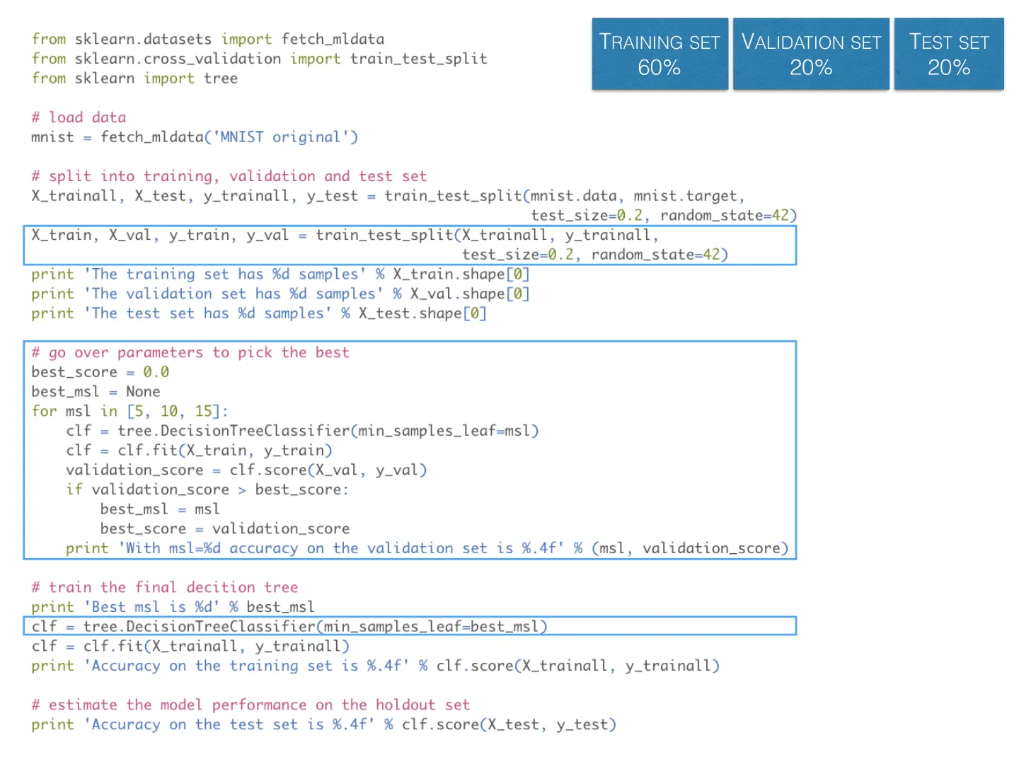
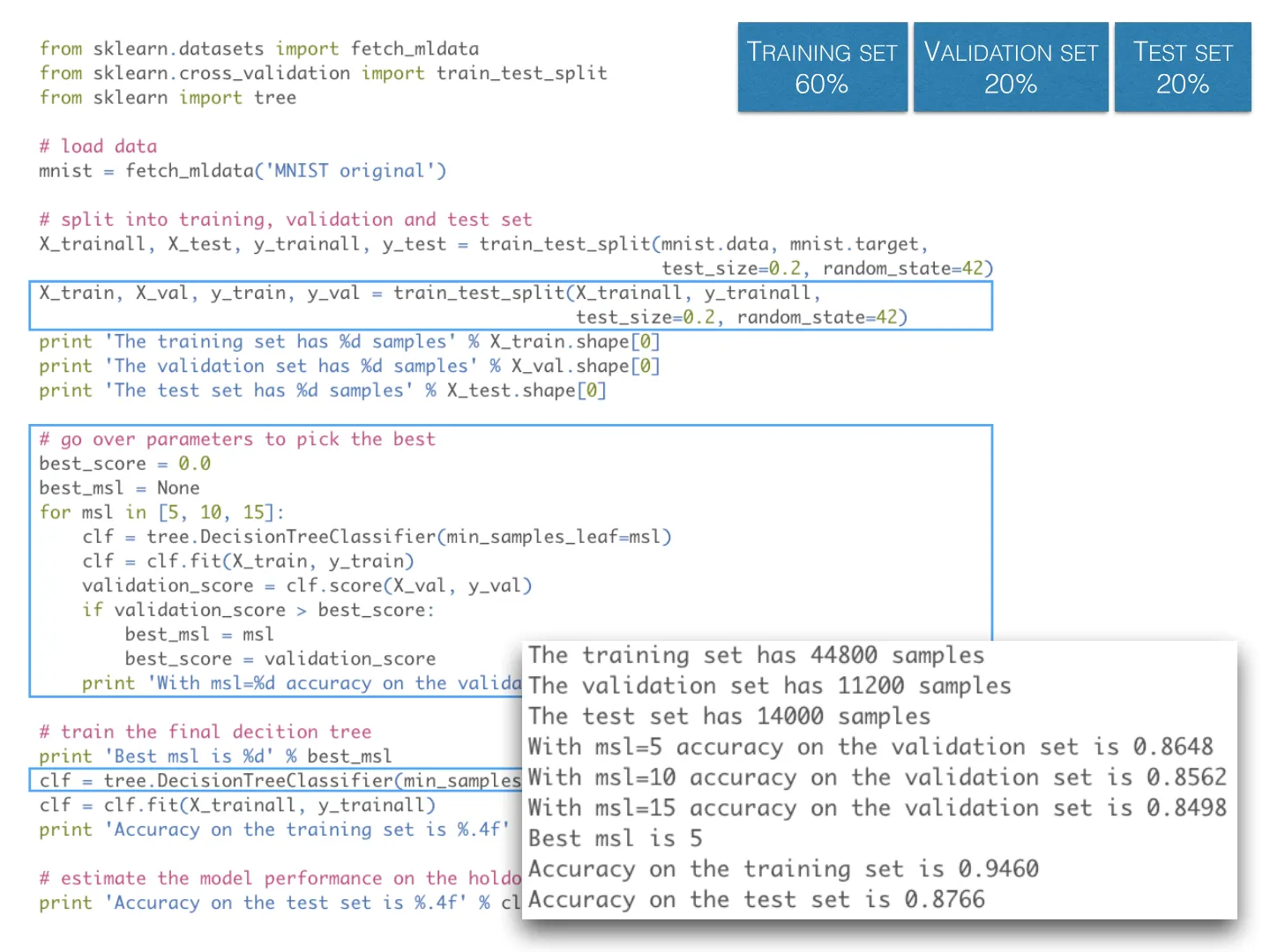
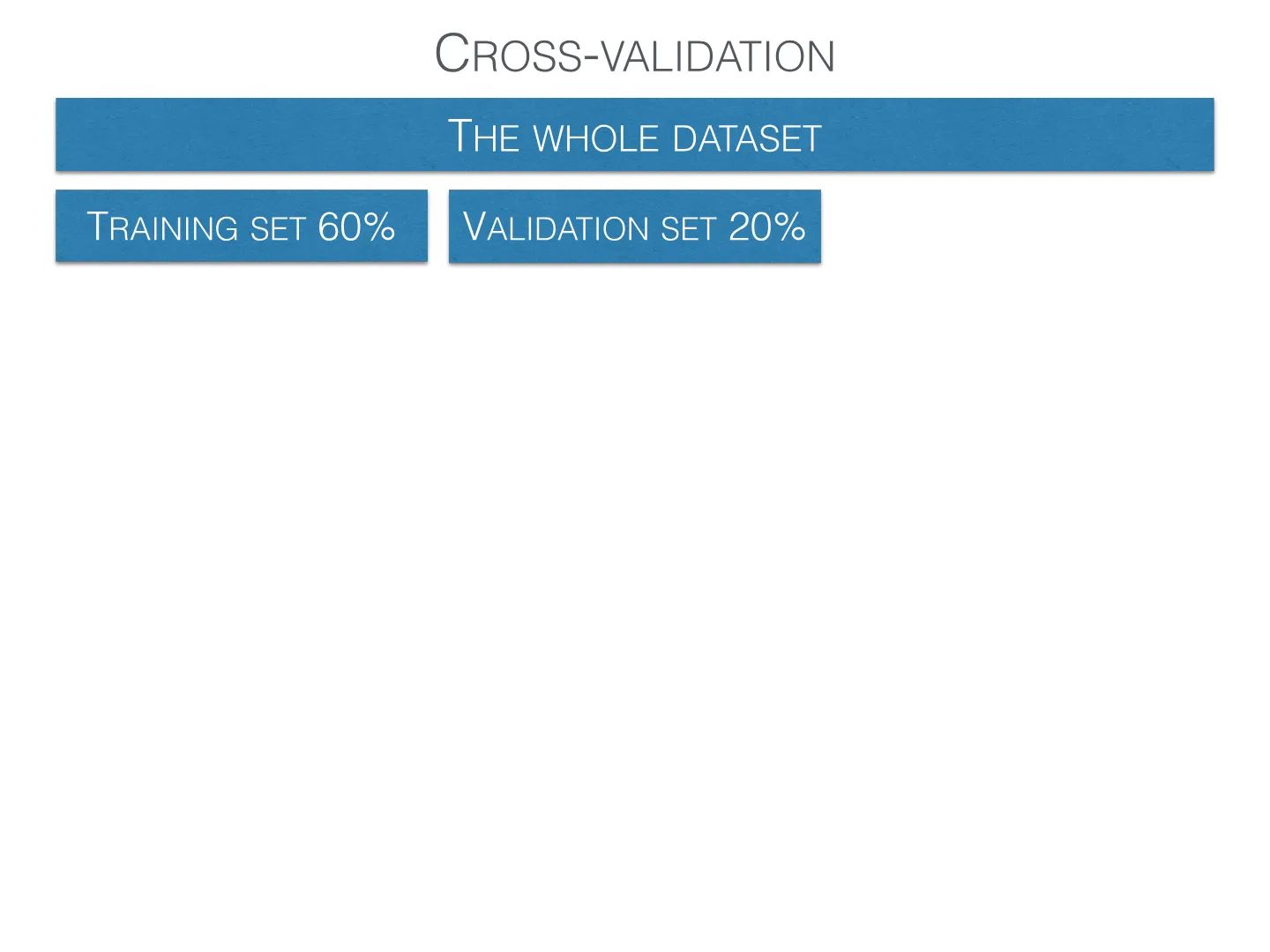
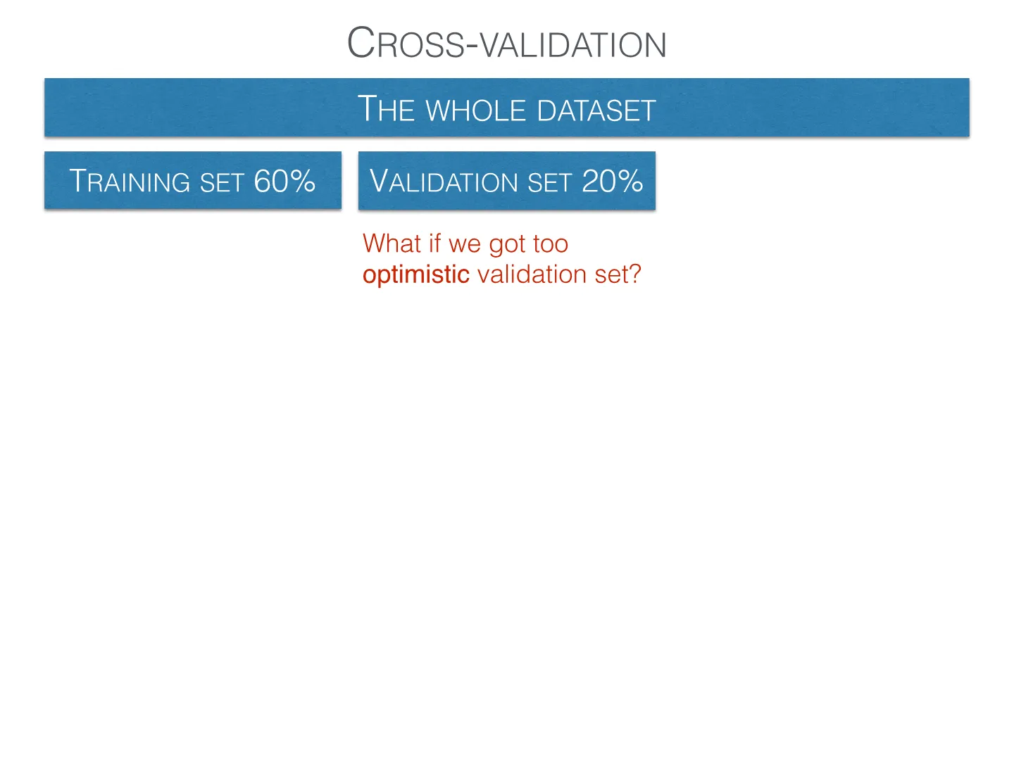
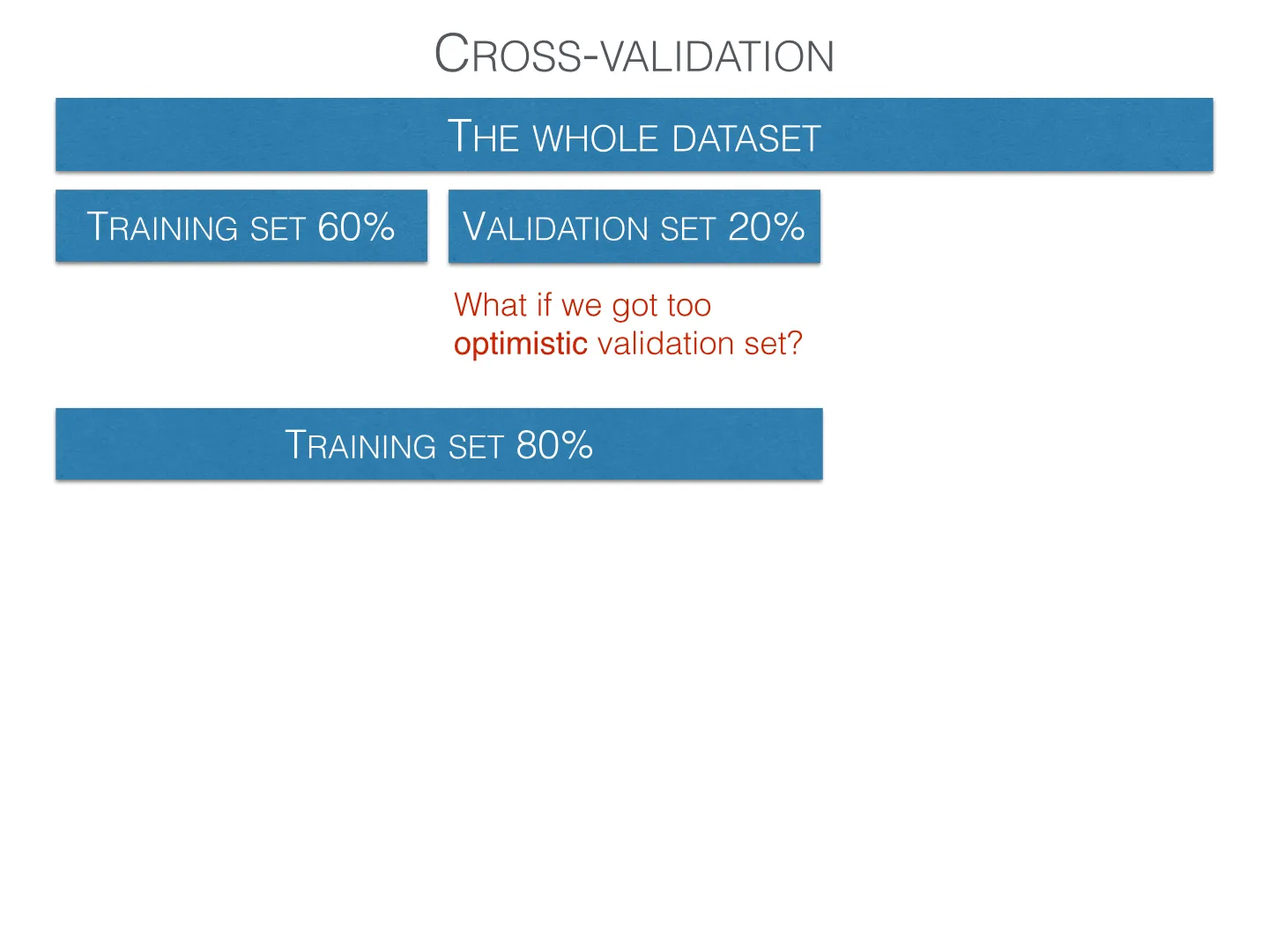
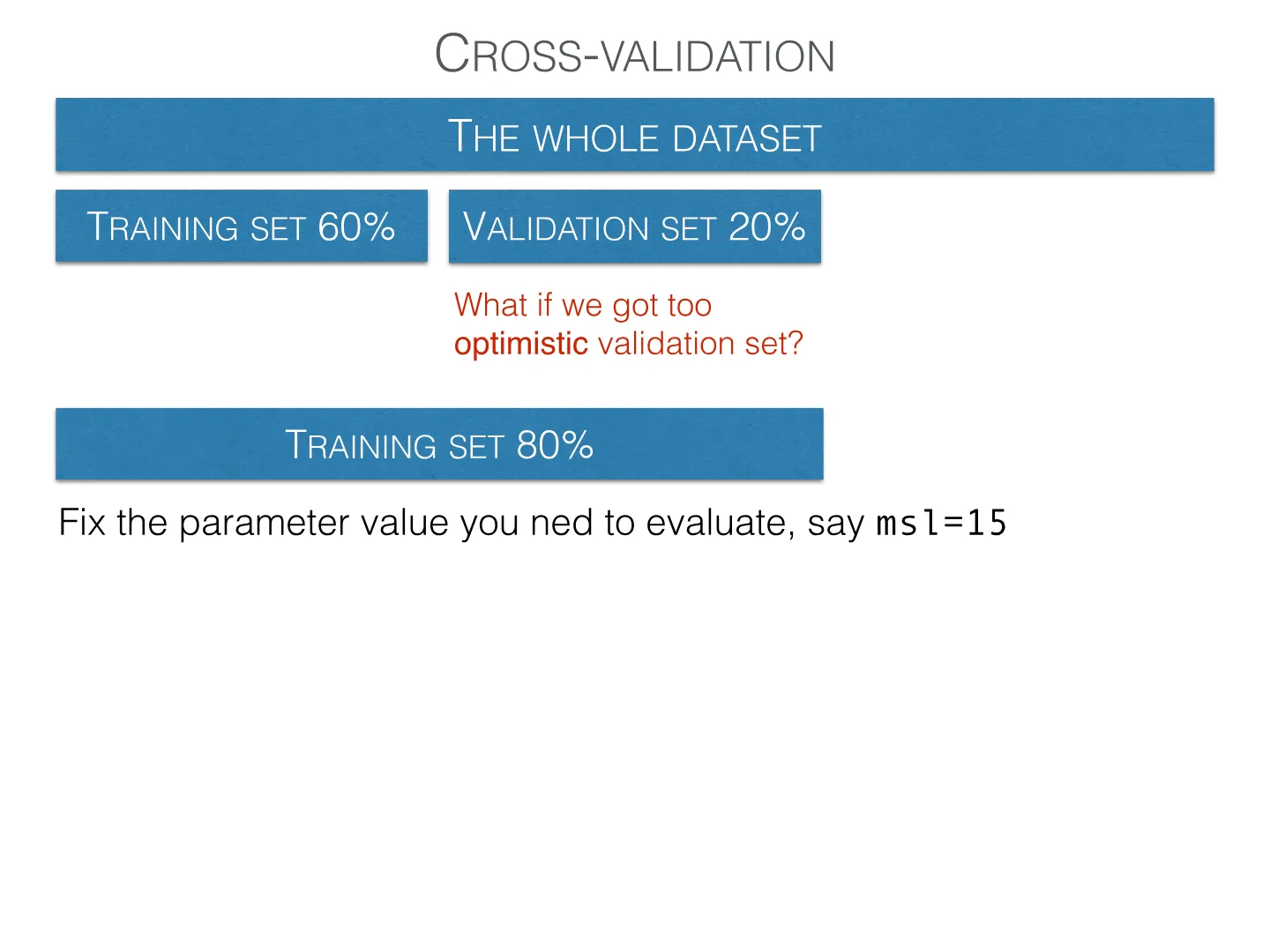
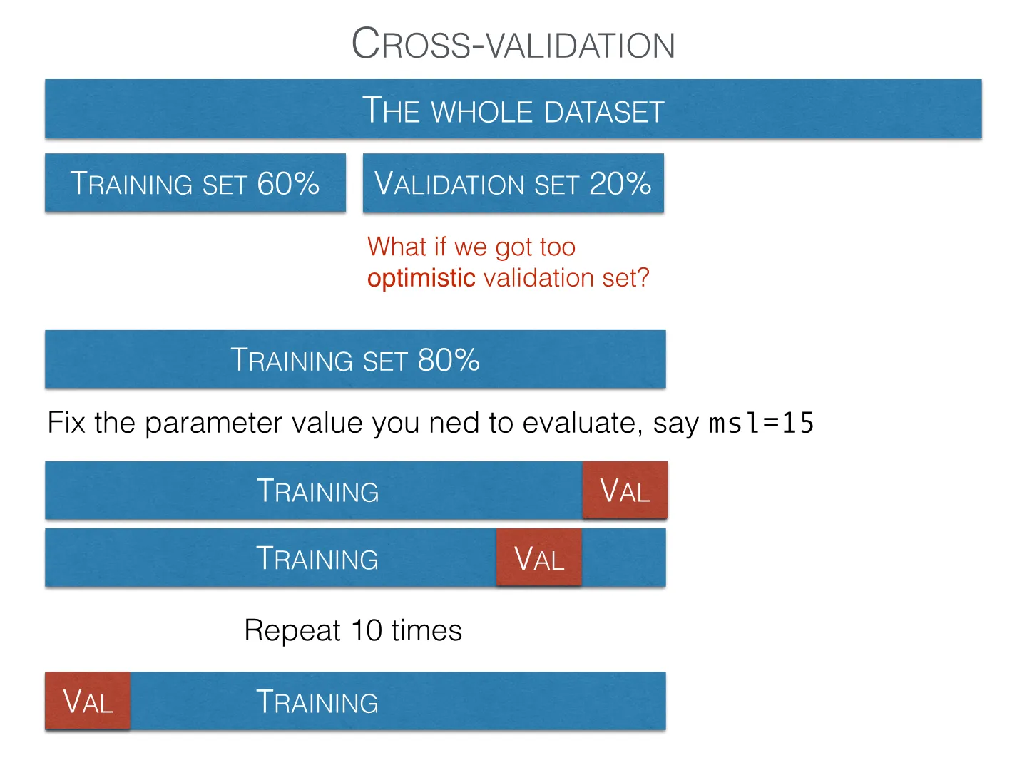
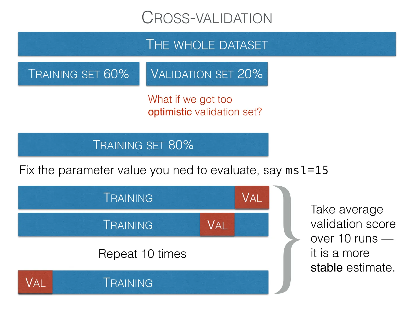
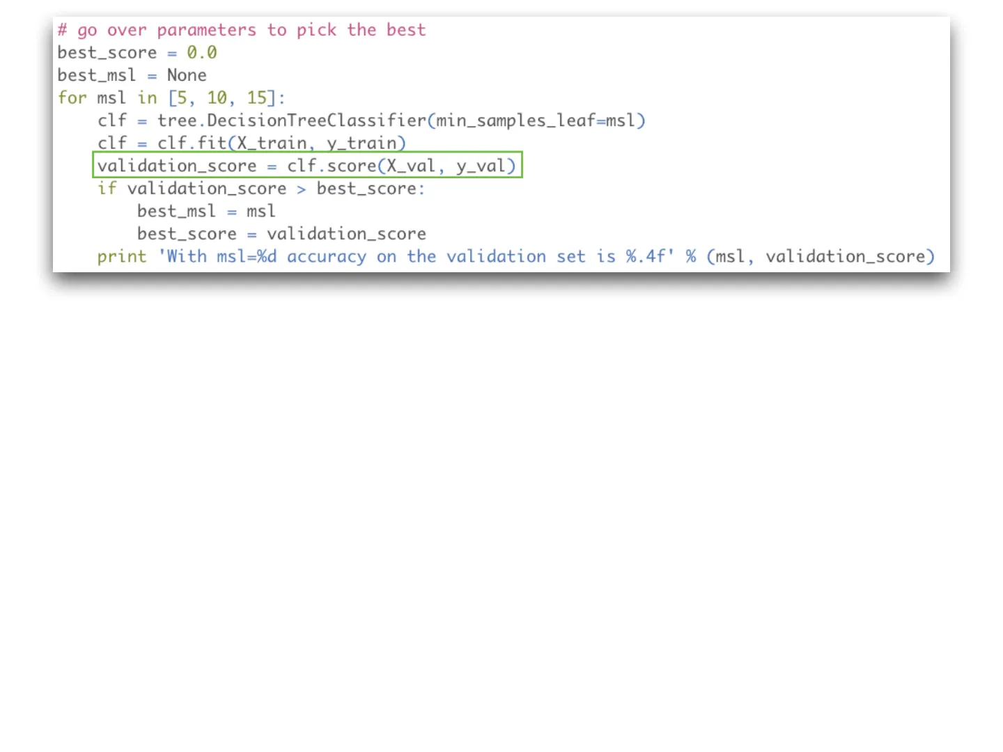
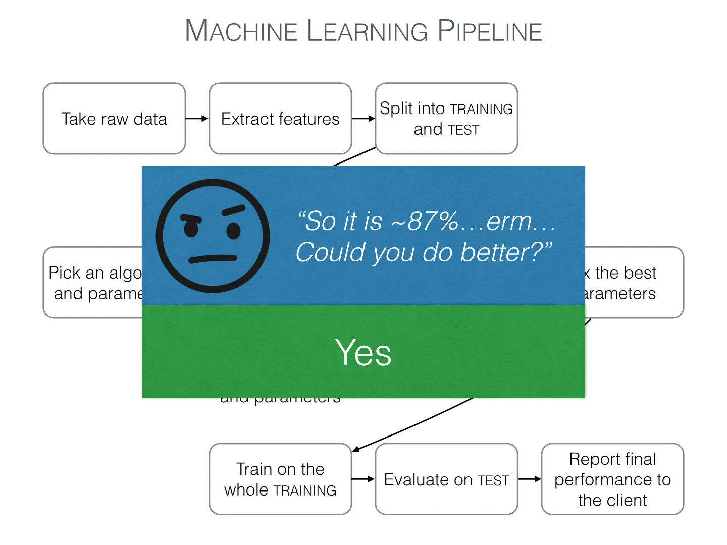
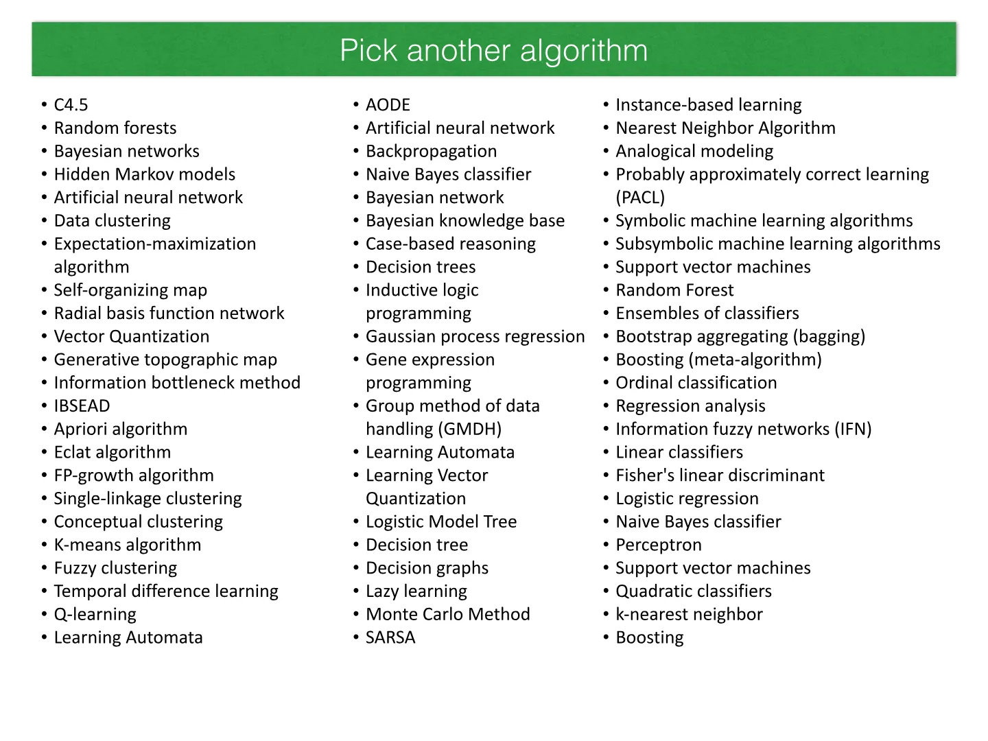
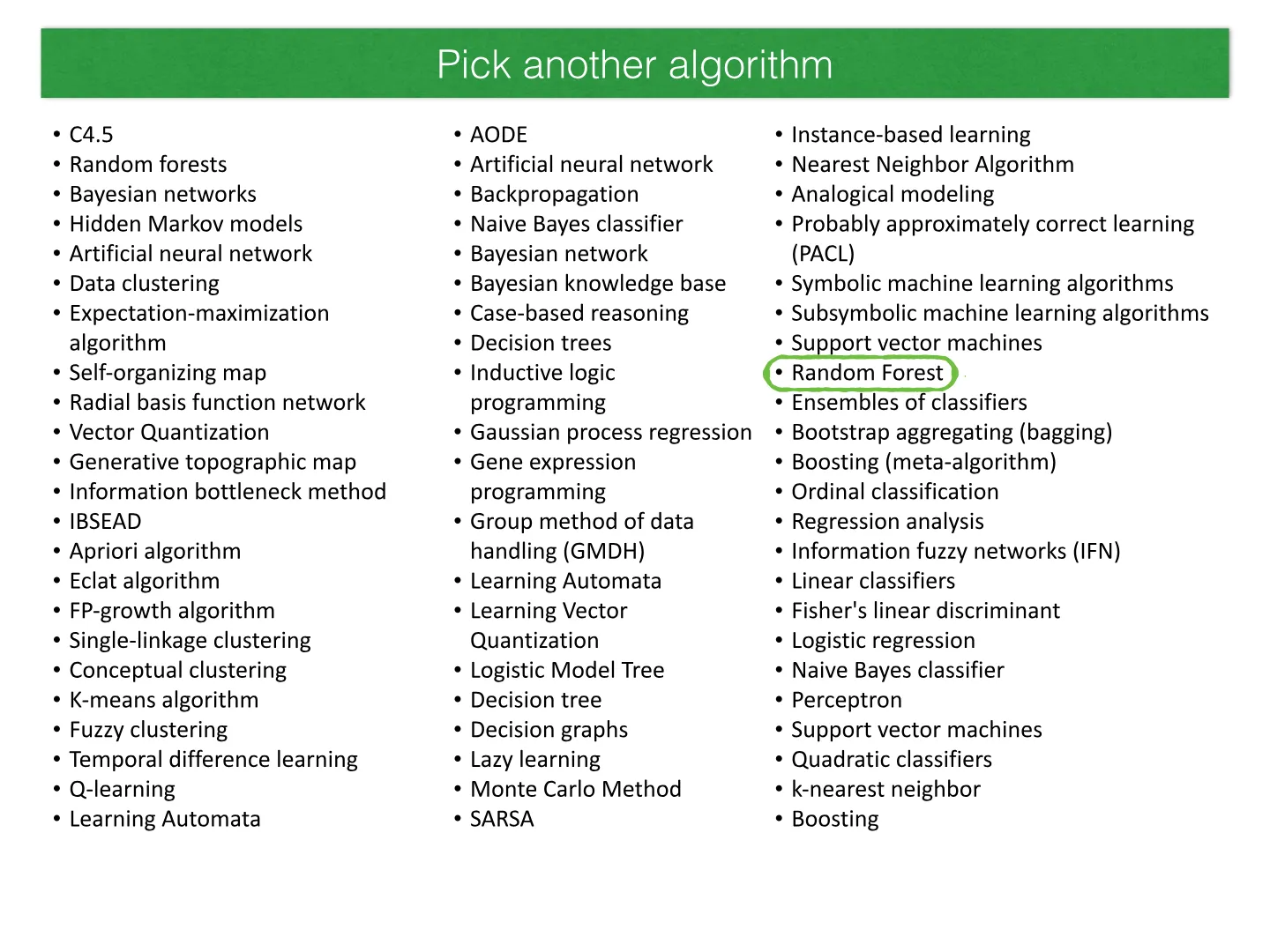
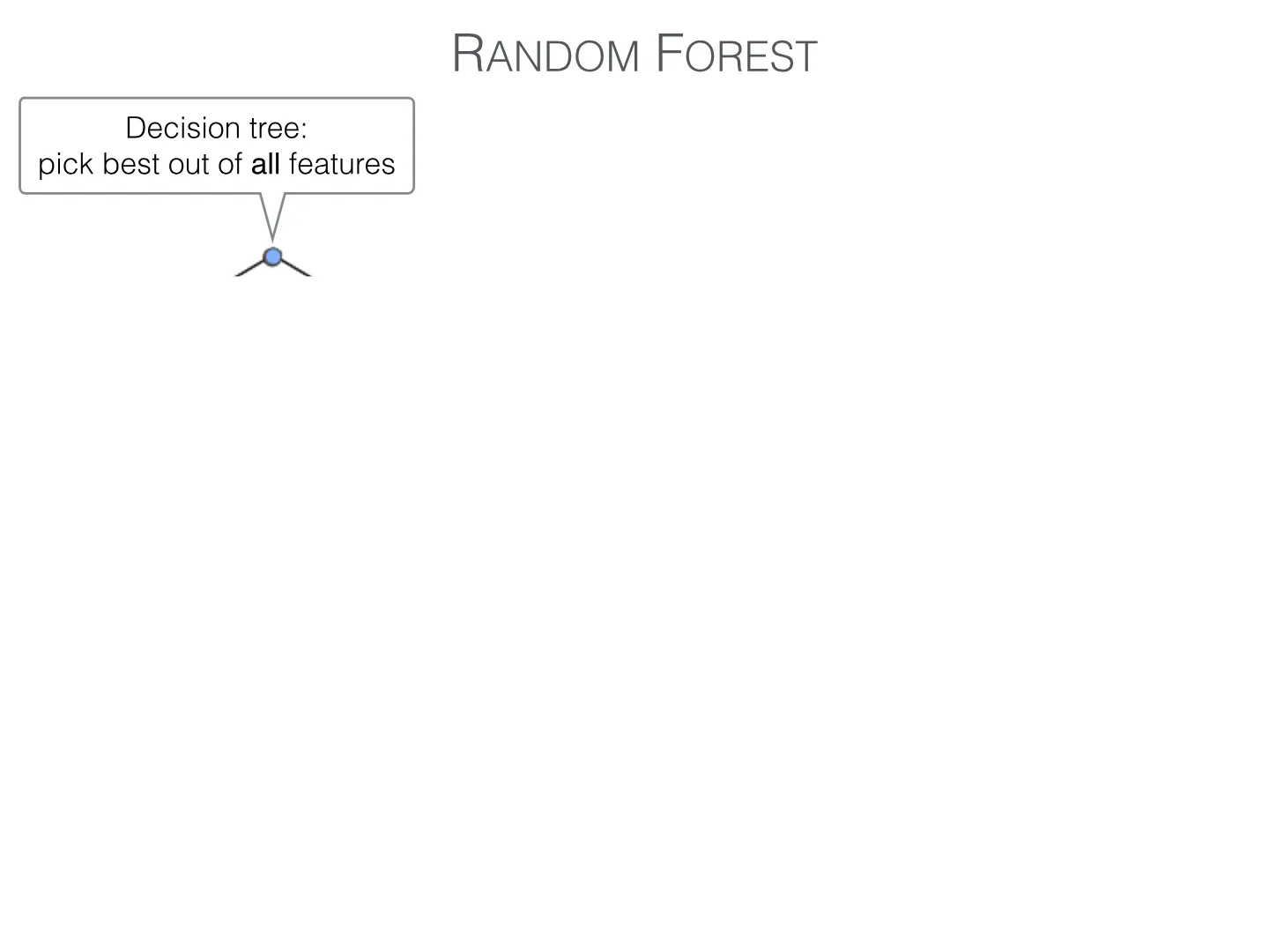
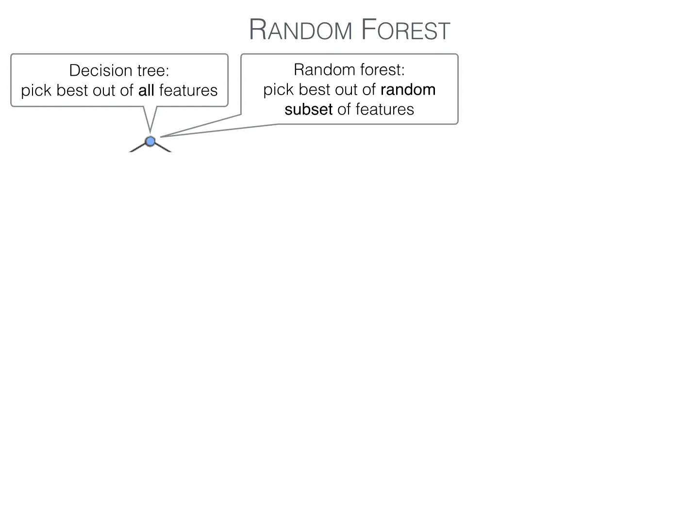
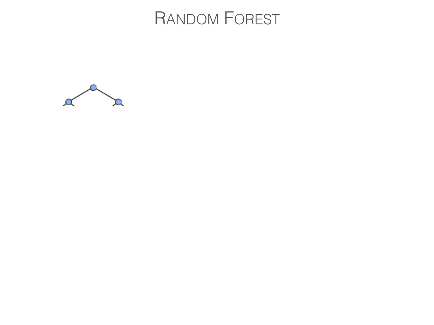
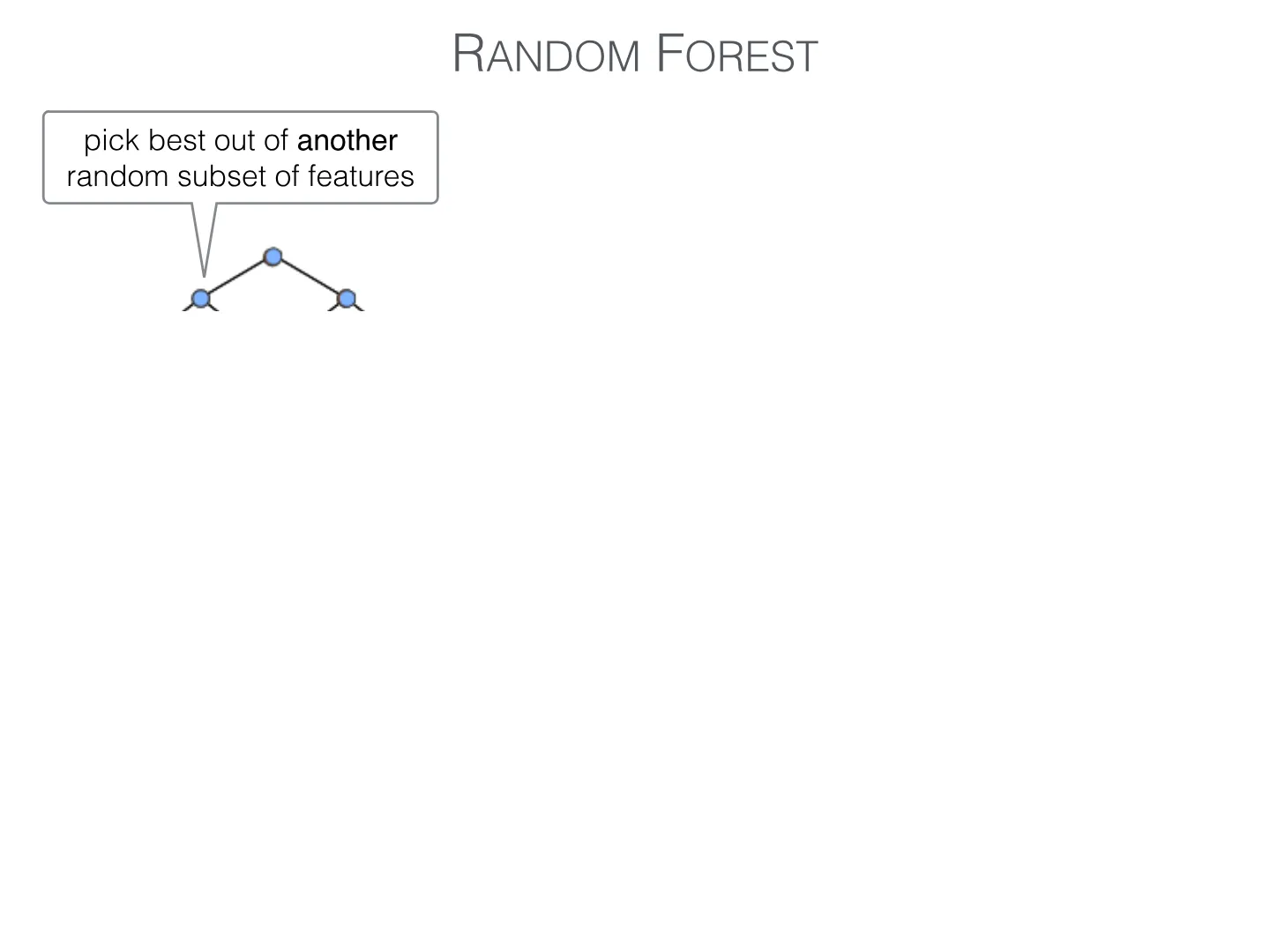
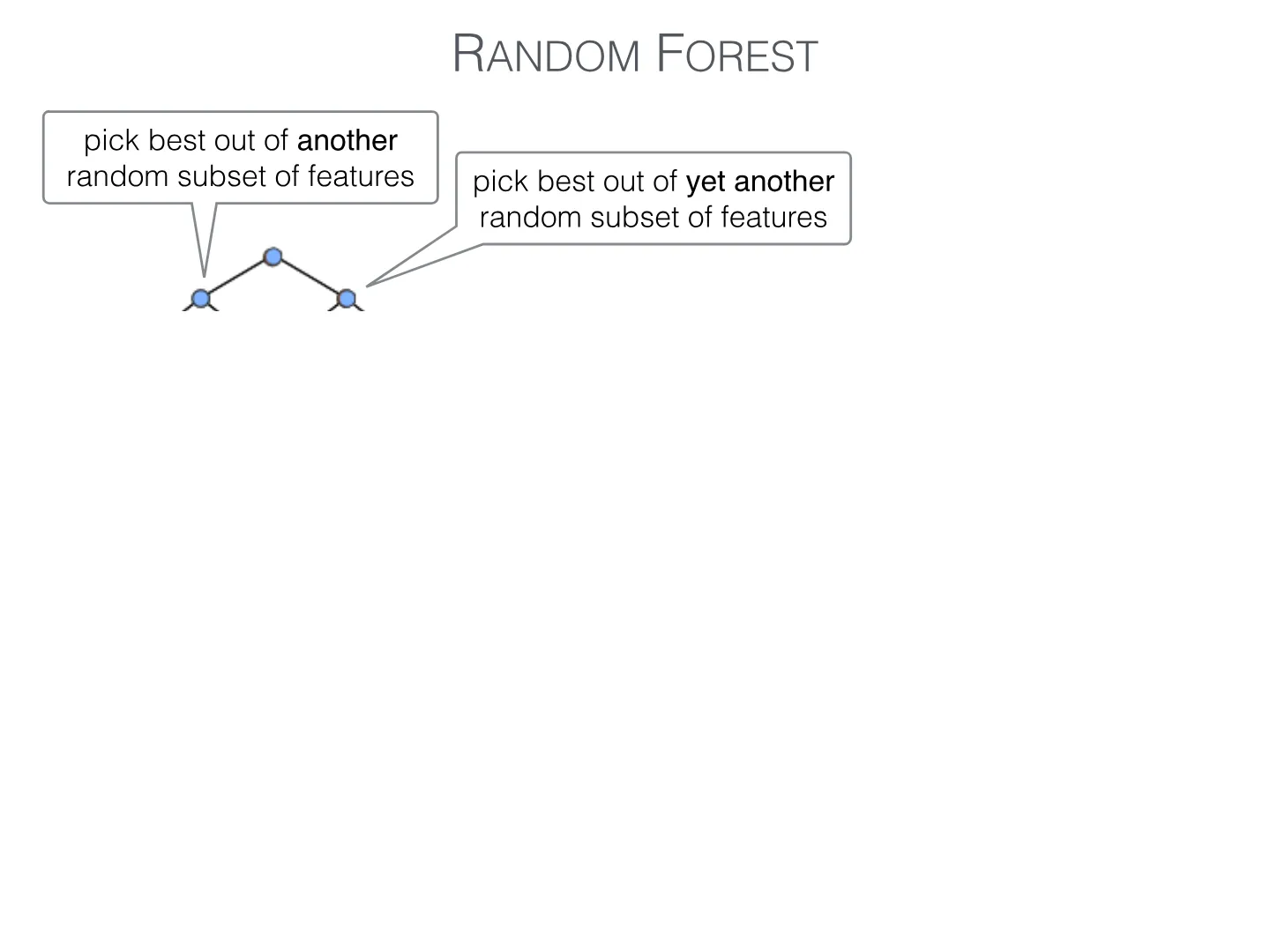
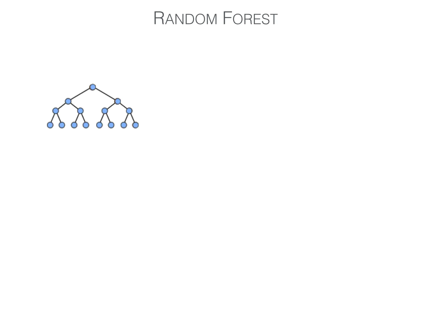
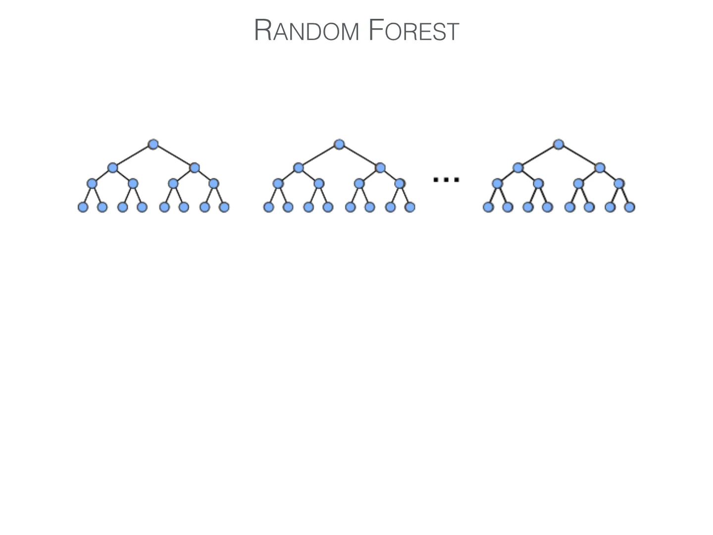
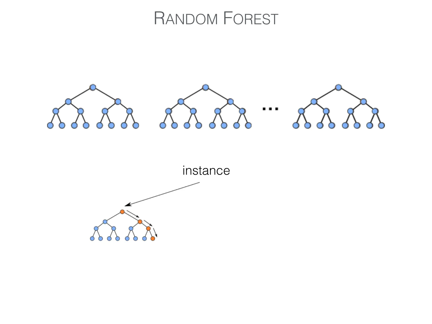
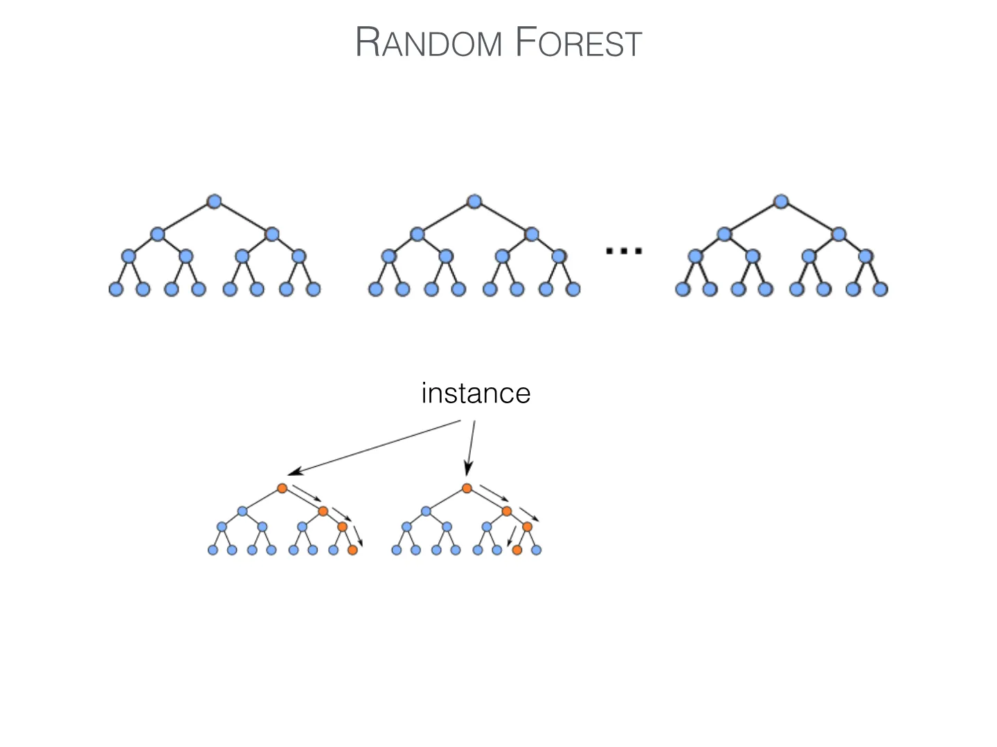
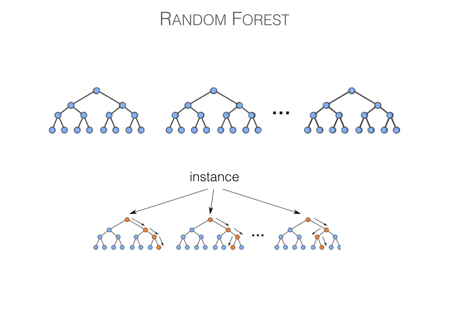
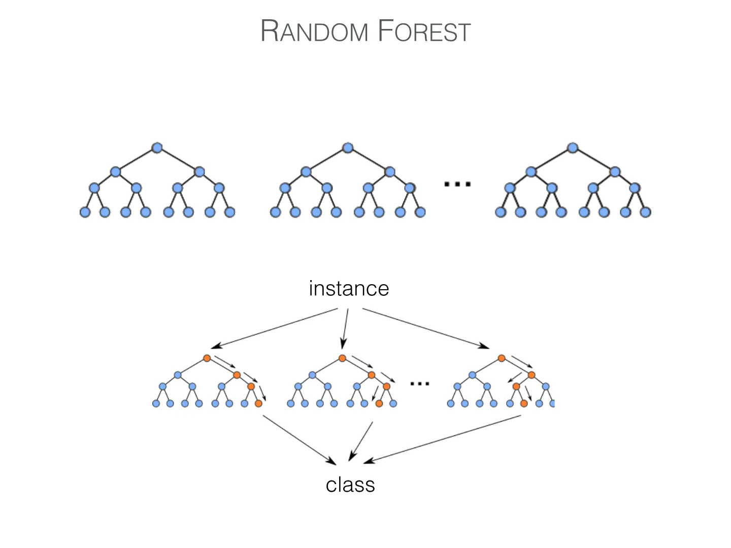
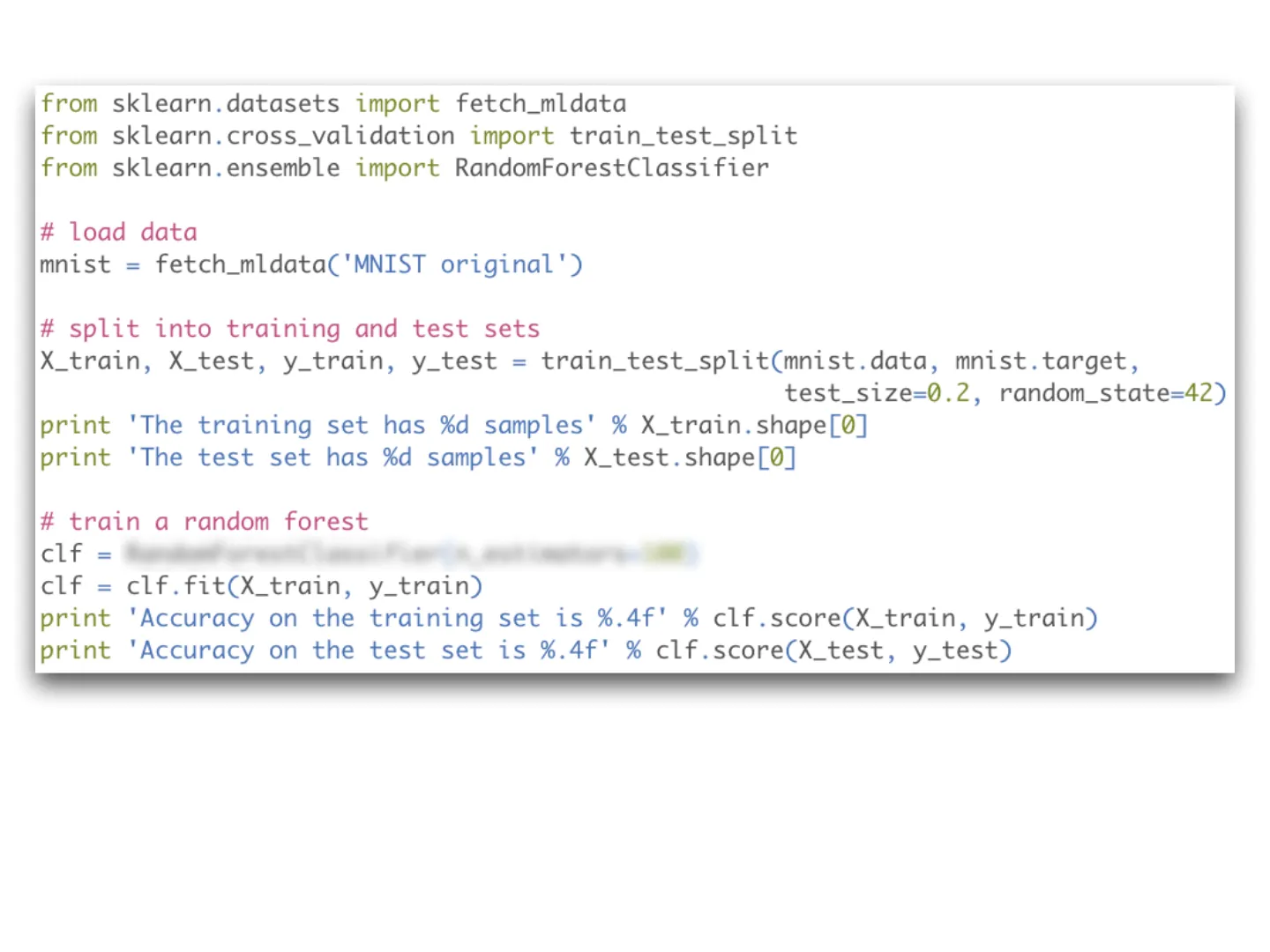
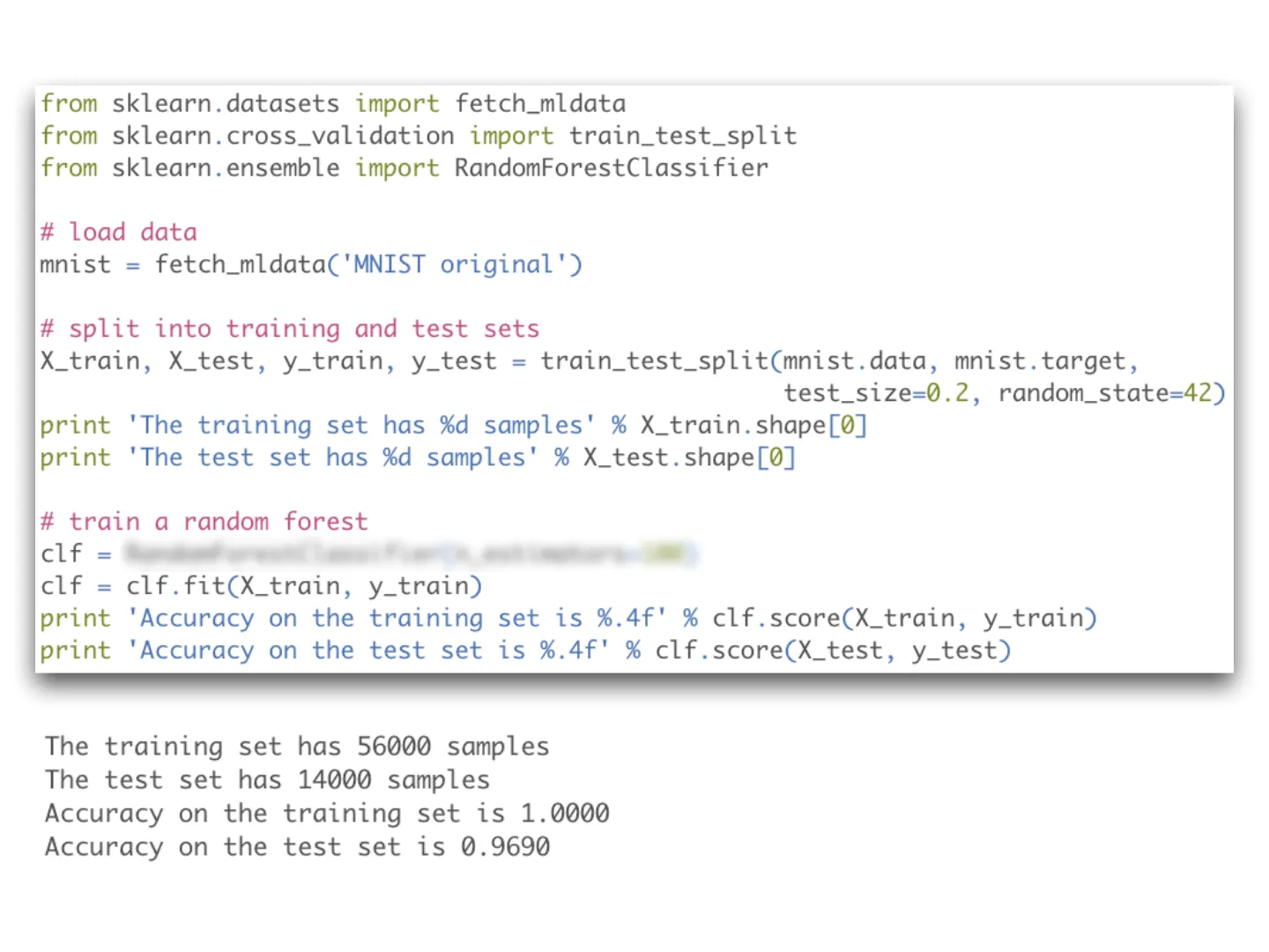
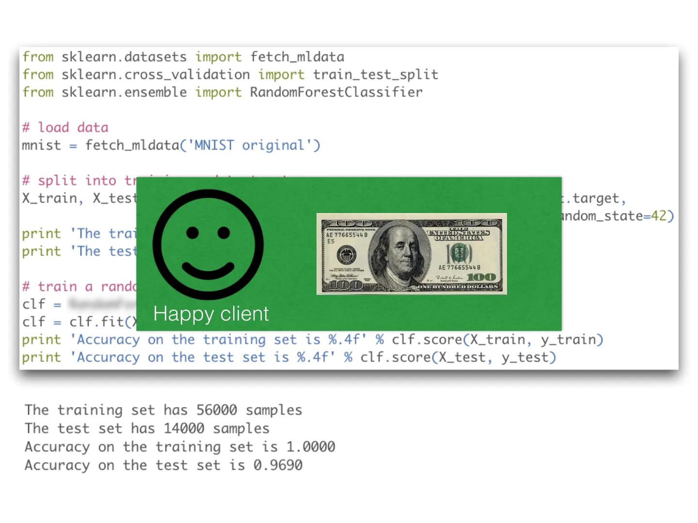
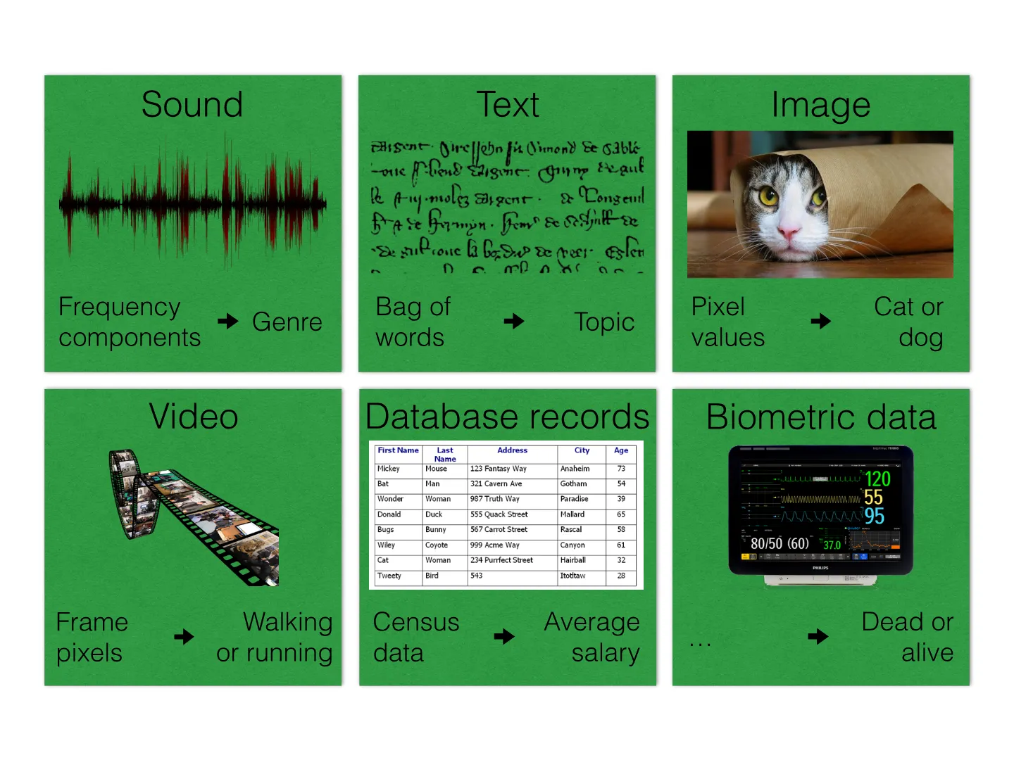
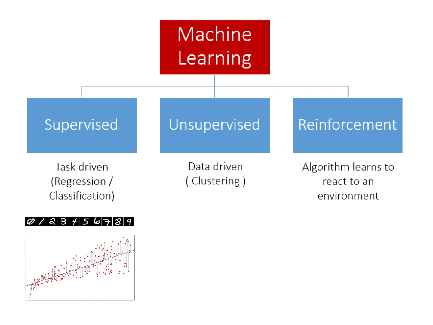
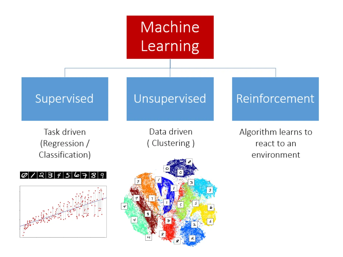
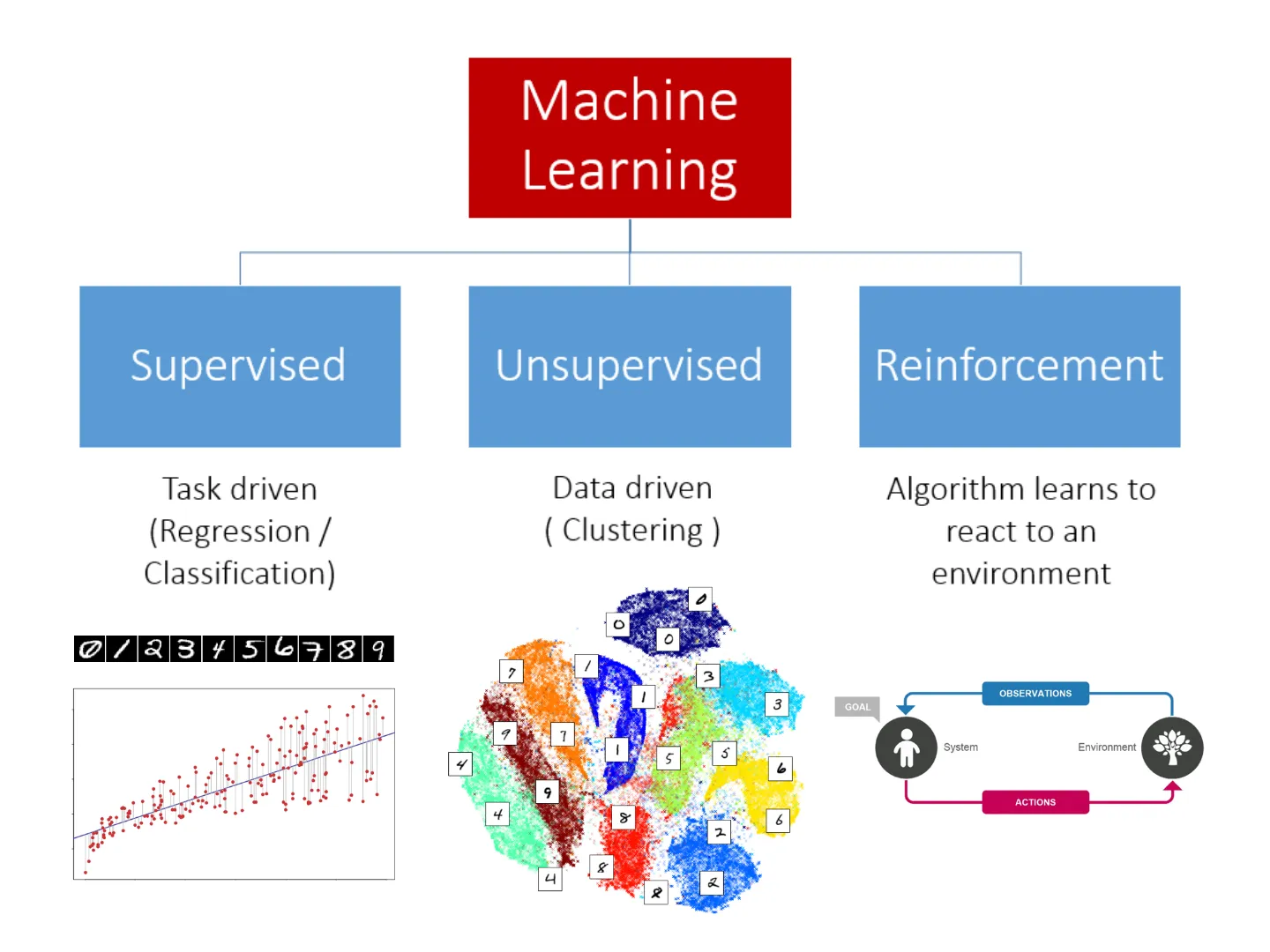
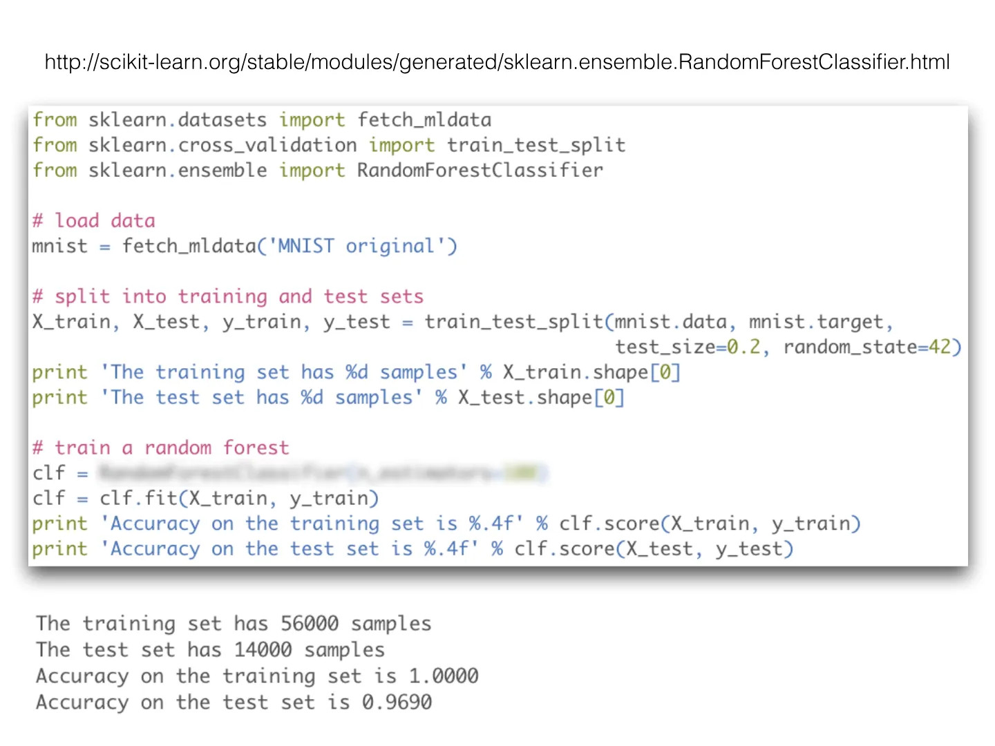
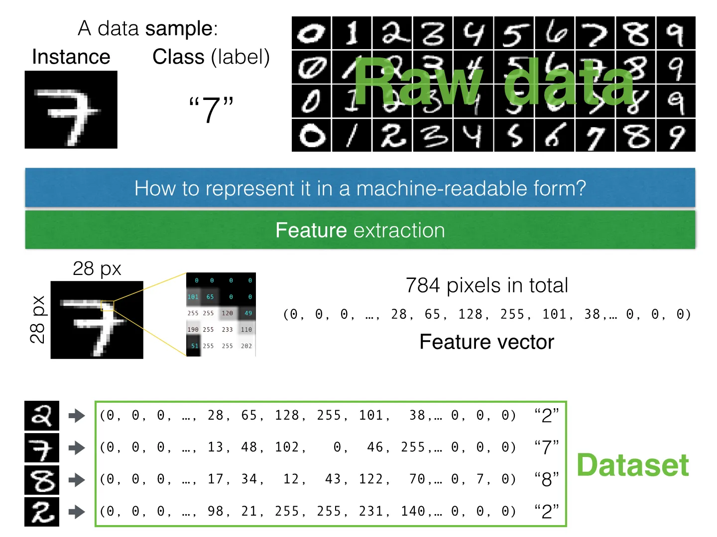
Slide 1 of 103: by Ilya Kuzovkin ilya.kuzovkin@gmail.com Mooncascade ML Camp 2016 Machine Learning ESSENTIAL CONCEPTSSlide 2 of 103: ONE MACHINE LEARNING USE CASESlide 3 of 103Slide 4 of 103Slide 5 of 103Slide 6 of 103Slide 7 of 103Slide 8 of 103Slide 9 of 103Slide 10 of 103: Can we ask a computer to create those patterns automatically ?Slide 11 of 103: Can we ask a computer to create those patterns automatically ? YesSlide 12 of 103: Can we ask a computer to create those patterns automatically ? Yes How?Slide 13 of 103: Raw dataSlide 14 of 103: Instance Raw data Class (label) A data sample : “7”Slide 15 of 103: Instance Raw data Class (label) A data sample : “7” How to represent it in a machine-readable form?Slide 16 of 103: Instance Raw data Class (label) A data sample : “7” How to represent it in a machine-readable form? Feature extractionSlide 17 of 103: Instance Raw data Class (label) A data sample : “7” How to represent it in a machine-readable form? Feature extraction 28 px 28 pxSlide 18 of 103: Instance Raw data Class (label) A data sample : “7” 28 px 28 px 784 pixels in total Feature vector (0, 0, 0, …, 28, 65, 128, 255, 101, 38,… 0, 0, 0) How to represent it in a machine-readable form? Feature extractionSlide 19 of 103: Instance Raw data Class (label) A data sample : “7” 28 px 28 px 784 pixels in total Feature vector (0, 0, 0, …, 28, 65, 128, 255, 101, 38,… 0, 0, 0) How to represent it in a machine-readable form? Feature extraction (0, 0, 0, …, 28, 65, 128, 255, 101, 38,… 0, 0, 0) (0, 0, 0, …,…Slide 20 of 103: Instance Raw data Class (label) A data sample : “7” 28 px 28 px 784 pixels in total Feature vector (0, 0, 0, …, 28, 65, 128, 255, 101, 38,… 0, 0, 0) How to represent it in a machine-readable form? Feature extraction (0, 0, 0, …, 28, 65, 128, 255, 101, 38,… 0, 0, 0) (0, 0, 0, …,…Slide 21 of 103: The data is in the right format — what’s next?Slide 22 of 103: The data is in the right format — what’s next? • C4.5 • Random forests • Bayesian networks • Hidden Markov models • Artificial neural network • Data clustering • Expectation-maximization algorithm • Self-organizing map • Radial basis function network • Vector Quantization •…Slide 23 of 103: The data is in the right format — what’s next? • C4.5 • Random forests • Bayesian networks • Hidden Markov models • Artificial neural network • Data clustering • Expectation-maximization algorithm • Self-organizing map • Radial basis function network • Vector Quantization •…Slide 24 of 103: DECISION TREE vs.Slide 25 of 103: DECISION TREE vs. (0, …, 28, 65, …, 207, 101, 0, 0) (0, …, 19, 34, …, 254, 54, 0, 0) (0, …, 87, 59, …, 240, 52, 4, 0) (0, …, 87, 52, …, 240, 19, 3, 0) (0, …, 28, 64, …, 102, 101, 0, 0) (0, …, 19, 23, …, 105, 54, 0, 0) (0, …, 87, 74, …, 121, 51, 7, 0) (0, …, 87, 112, …, 239, 52,…Slide 26 of 103: DECISION TREE vs. (0, …, 28, 65, …, 207, 101, 0, 0) (0, …, 19, 34, …, 254, 54, 0, 0) (0, …, 87, 59, …, 240, 52, 4, 0) (0, …, 87, 52, …, 240, 19, 3, 0) (0, …, 28, 64, …, 102, 101, 0, 0) (0, …, 19, 23, …, 105, 54, 0, 0) (0, …, 87, 74, …, 121, 51, 7, 0) (0, …, 87, 112, …, 239, 52,…Slide 27 of 103: DECISION TREE vs. (0, …, 28, 65, …, 207, 101, 0, 0) (0, …, 19, 34, …, 254, 54, 0, 0) (0, …, 87, 59, …, 240, 52, 4, 0) (0, …, 87, 52, …, 240, 19, 3, 0) (0, …, 28, 64, …, 102, 101, 0, 0) (0, …, 19, 23, …, 105, 54, 0, 0) (0, …, 87, 74, …, 121, 51, 7, 0) (0, …, 87, 112, …, 239, 52,…Slide 28 of 103: DECISION TREE vs. (0, …, 28, 65, …, 207, 101, 0, 0) (0, …, 19, 34, …, 254, 54, 0, 0) (0, …, 87, 59, …, 240, 52, 4, 0) (0, …, 87, 52, …, 240, 19, 3, 0) (0, …, 28, 64, …, 102, 101, 0, 0) (0, …, 19, 23, …, 105, 54, 0, 0) (0, …, 87, 74, …, 121, 51, 7, 0) (0, …, 87, 112, …, 239, 52,…Slide 29 of 103: DECISION TREE vs. (0, …, 28, 65, …, 207, 101, 0, 0) (0, …, 19, 34, …, 254, 54, 0, 0) (0, …, 87, 59, …, 240, 52, 4, 0) (0, …, 87, 52, …, 240, 19, 3, 0) (0, …, 28, 64, …, 102, 101, 0, 0) (0, …, 19, 23, …, 105, 54, 0, 0) (0, …, 87, 74, …, 121, 51, 7, 0) (0, …, 87, 112, …, 239, 52,…Slide 30 of 103: DECISION TREE vs. (0, …, 28, 65, …, 207, 101, 0, 0) (0, …, 19, 34, …, 254, 54, 0, 0) (0, …, 87, 59, …, 240, 52, 4, 0) (0, …, 87, 52, …, 240, 19, 3, 0) (0, …, 28, 64, …, 102, 101, 0, 0) (0, …, 19, 23, …, 105, 54, 0, 0) (0, …, 87, 74, …, 121, 51, 7, 0) (0, …, 87, 112, …, 239, 52,…Slide 31 of 103: DECISION TREE vs. (0, …, 28, 65, …, 207, 101, 0, 0) (0, …, 19, 34, …, 254, 54, 0, 0) (0, …, 87, 59, …, 240, 52, 4, 0) (0, …, 87, 52, …, 240, 19, 3, 0) (0, …, 28, 64, …, 102, 101, 0, 0) (0, …, 19, 23, …, 105, 54, 0, 0) (0, …, 87, 74, …, 121, 51, 7, 0) (0, …, 87, 112, …, 239, 52,…Slide 32 of 103: DECISION TREE vs. (0, …, 28, 65, …, 207, 101, 0, 0) (0, …, 19, 34, …, 254, 54, 0, 0) (0, …, 87, 59, …, 240, 52, 4, 0) (0, …, 87, 52, …, 240, 19, 3, 0) (0, …, 28, 64, …, 102, 101, 0, 0) (0, …, 19, 23, …, 105, 54, 0, 0) (0, …, 87, 74, …, 121, 51, 7, 0) (0, …, 87, 112, …, 239, 52,…Slide 33 of 103: DECISION TREESlide 34 of 103: DECISION TREESlide 35 of 103: ACCURACYSlide 36 of 103: ACCURACY Confusion matrix True class Predicted classSlide 37 of 103: ACCURACY Confusion matrix acc = correctly classified total number of samples True class Predicted classSlide 38 of 103: ACCURACY Confusion matrix acc = correctly classified total number of samples Beware of an imbalanced dataset! True class Predicted classSlide 39 of 103: ACCURACY Confusion matrix acc = correctly classified total number of samples Beware of an imbalanced dataset! Consider the following model: “Always predict 2” True class Predicted classSlide 40 of 103: ACCURACY Confusion matrix acc = correctly classified total number of samples Beware of an imbalanced dataset! Consider the following model: “Always predict 2” Accuracy 0.9 True class Predicted classSlide 41 of 103: DECISION TREESlide 42 of 103: DECISION TREE “You said 100% accurate?! Every 10th digit your system detects is wrong!” Angry clientSlide 43 of 103: DECISION TREE “You said 100% accurate?! Every 10th digit your system detects is wrong!” Angry client We’ve trained our system on the data the client gave us. But our system has never seen the new data the client applied it to. And in the real life — it never will…Slide 44 of 103: OVERFITTING Simulate the real-life situation — split the datasetSlide 45 of 103: OVERFITTING Simulate the real-life situation — split the datasetSlide 46 of 103: OVERFITTING Simulate the real-life situation — split the datasetSlide 47 of 103: OVERFITTING Simulate the real-life situation — split the datasetSlide 48 of 103: Underfitting ! “Too stupid” OK Overfitting ! “Too smart” OVERFITTINGSlide 49 of 103: Underfitting ! “Too stupid” OK Overfitting ! “Too smart” OVERFITTING Our current decision tree has too much capacity, it just has memorized all of the data. Let’s make it less complex.Slide 50 of 103Slide 51 of 103Slide 52 of 103Slide 53 of 103: You probably did not notice, but we are overfitting again :(Slide 54 of 103: TEST SET 20% TRAINING SET 60% THE WHOLE DATASET VALIDATION SET 20%Slide 55 of 103: TEST SET 20% TRAINING SET 60% THE WHOLE DATASET VALIDATION SET 20% Fit various models and parameter combinations on this subsetSlide 56 of 103: TEST SET 20% TRAINING SET 60% THE WHOLE DATASET VALIDATION SET 20% Fit various models and parameter combinations on this subset • Evaluate the models created with different parametersSlide 57 of 103: TEST SET 20% TRAINING SET 60% THE WHOLE DATASET VALIDATION SET 20% Fit various models and parameter combinations on this subset • Evaluate the models created with different parameters ! • Estimate overfitting TRA VALISlide 58 of 103: TEST SET 20% TRAINING SET 60% THE WHOLE DATASET VALIDATION SET 20% Fit various models and parameter combinations on this subset • Evaluate the models created with different parameters ! • Estimate overfitting TRA VALI TRA VALISlide 59 of 103: TEST SET 20% TRAINING SET 60% THE WHOLE DATASET VALIDATION SET 20% Fit various models and parameter combinations on this subset • Evaluate the models created with different parameters ! • Estimate overfitting TRA VALI TRA VALI TRA VALISlide 60 of 103: TEST SET 20% TRAINING SET 60% THE WHOLE DATASET VALIDATION SET 20% Fit various models and parameter combinations on this subset • Evaluate the models created with different parameters ! • Estimate overfitting TRA VALI TRA VALI TRA VALI TRA VALISlide 61 of 103: TEST SET 20% TRAINING SET 60% THE WHOLE DATASET VALIDATION SET 20% Fit various models and parameter combinations on this subset • Evaluate the models created with different parameters ! • Estimate overfitting TRA VALI TRA VALI TRA VALI TRA VALI TRA VALISlide 62 of 103: TEST SET 20% TRAINING SET 60% THE WHOLE DATASET VALIDATION SET 20% Fit various models and parameter combinations on this subset • Evaluate the models created with different parameters ! • Estimate overfitting Use only once to get the final performance estimate TRA VALI TRA VALI…Slide 63 of 103: TEST SET 20% TRAINING SET 60% VALIDATION SET 20%Slide 64 of 103: TEST SET 20% TRAINING SET 60% VALIDATION SET 20%Slide 65 of 103: CROSS-VALIDATION TRAINING SET 60% THE WHOLE DATASET VALIDATION SET 20%Slide 66 of 103: CROSS-VALIDATION TRAINING SET 60% THE WHOLE DATASET VALIDATION SET 20% What if we got too optimistic validation set?Slide 67 of 103: CROSS-VALIDATION TRAINING SET 60% THE WHOLE DATASET VALIDATION SET 20% What if we got too optimistic validation set? TRAINING SET 80%Slide 68 of 103: CROSS-VALIDATION TRAINING SET 60% THE WHOLE DATASET VALIDATION SET 20% What if we got too optimistic validation set? TRAINING SET 80% Fix the parameter value you ned to evaluate, say msl=15Slide 69 of 103: CROSS-VALIDATION TRAINING SET 60% THE WHOLE DATASET VALIDATION SET 20% What if we got too optimistic validation set? TRAINING SET 80% Fix the parameter value you ned to evaluate, say msl=15 TRAINING VAL TRAINING VAL TRAINING VAL Repeat 10 timesSlide 70 of 103: CROSS-VALIDATION TRAINING SET 60% THE WHOLE DATASET VALIDATION SET 20% What if we got too optimistic validation set? TRAINING SET 80% Fix the parameter value you ned to evaluate, say msl=15 TRAINING VAL TRAINING VAL TRAINING VAL Repeat 10 times } Take average validation score…Slide 71 of 103Slide 72 of 103Slide 73 of 103Slide 74 of 103: MACHINE LEARNING PIPELINE Take raw data Extract features Split into TRAINING and TEST Pick an algorithm and parameters Train on the TRAINING data Evaluate on the TRAINING data with CV Train on the whole TRAINING Fix the best parameters Evaluate on TEST Report final performance…Slide 75 of 103: MACHINE LEARNING PIPELINE Take raw data Extract features Split into TRAINING and TEST Pick an algorithm and parameters Train on the TRAINING data Evaluate on the TRAINING data with CV Train on the whole TRAINING Fix the best parameters Evaluate on TEST Report final performance…Slide 76 of 103: MACHINE LEARNING PIPELINE Take raw data Extract features Split into TRAINING and TEST Pick an algorithm and parameters Train on the TRAINING data Evaluate on the TRAINING data with CV Train on the whole TRAINING Fix the best parameters Evaluate on TEST Report final performance…Slide 77 of 103: • C4.5 • Random forests • Bayesian networks • Hidden Markov models • Artificial neural network • Data clustering • Expectation-maximization algorithm • Self-organizing map • Radial basis function network • Vector Quantization • Generative topographic map • Information bottleneck…Slide 78 of 103: • C4.5 • Random forests • Bayesian networks • Hidden Markov models • Artificial neural network • Data clustering • Expectation-maximization algorithm • Self-organizing map • Radial basis function network • Vector Quantization • Generative topographic map • Information bottleneck…Slide 79 of 103: RANDOM FORESTSlide 80 of 103: RANDOM FOREST Decision tree: pick best out of all featuresSlide 81 of 103: RANDOM FOREST Decision tree: pick best out of all features Random forest: pick best out of random subset of featuresSlide 82 of 103: RANDOM FORESTSlide 83 of 103: RANDOM FOREST pick best out of another random subset of featuresSlide 84 of 103: RANDOM FOREST pick best out of another random subset of features pick best out of yet another random subset of featuresSlide 85 of 103: RANDOM FORESTSlide 86 of 103: RANDOM FORESTSlide 87 of 103: RANDOM FOREST class instanceSlide 88 of 103: RANDOM FOREST class instanceSlide 89 of 103: RANDOM FOREST class instanceSlide 90 of 103: RANDOM FOREST class instanceSlide 91 of 103Slide 92 of 103Slide 93 of 103: Happy clientSlide 94 of 103: ALL OTHER USE CASESSlide 95 of 103: Sound Frequency components Genre Bag of words Topic Text Pixel values Image Cat or dog Video Frame pixels Walking or running Database records Biometric data Census data Average salary … Dead or aliveSlide 96 of 103Slide 97 of 103Slide 98 of 103Slide 99 of 103Slide 100 of 103Slide 101 of 103: HANDS-ON SESSIONSlide 102 of 103: http://scikit-learn.org/stable/modules/generated/sklearn.ensemble.RandomForestClassifier.htmlSlide 103 of 103
1 / 103

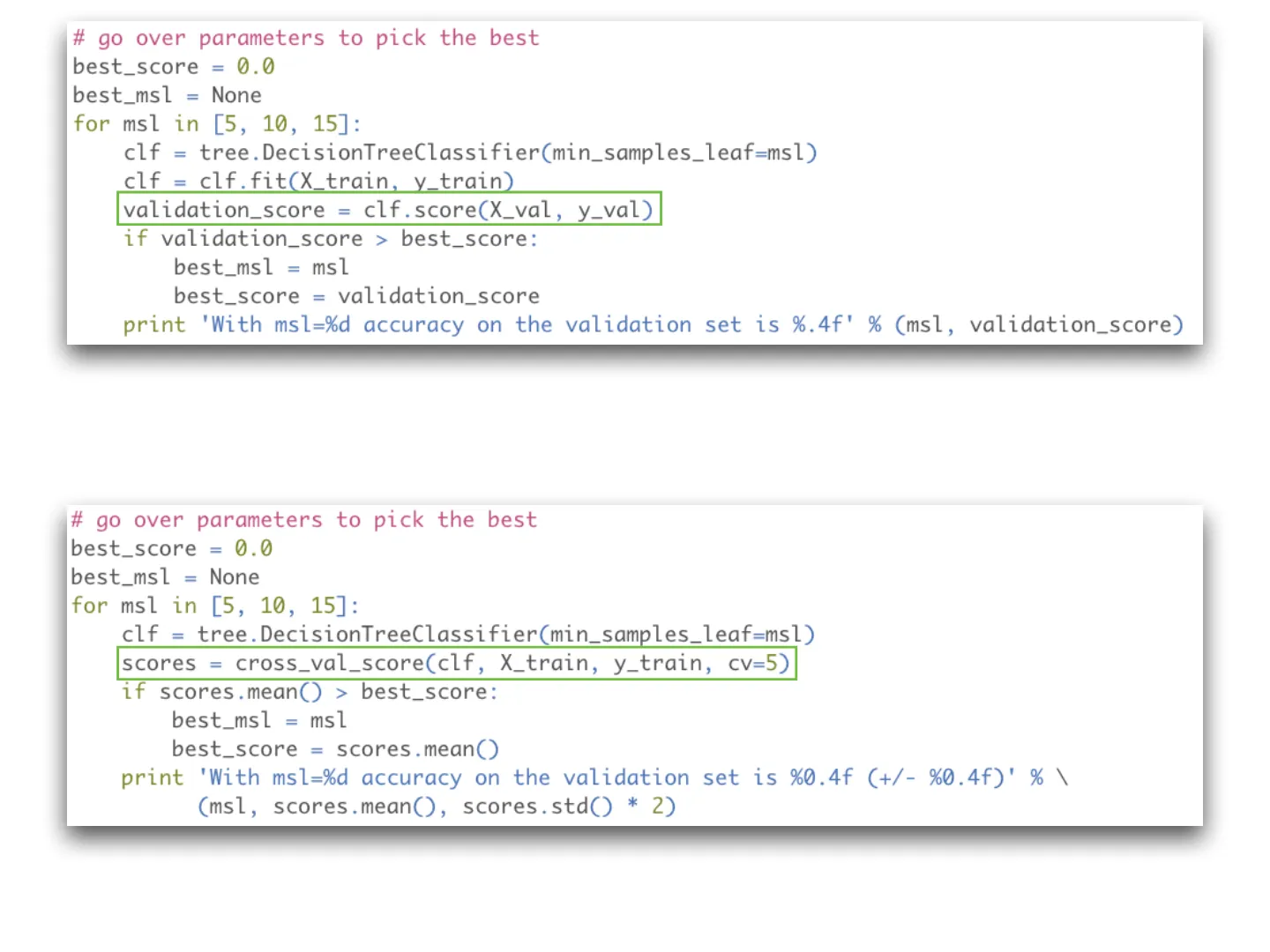
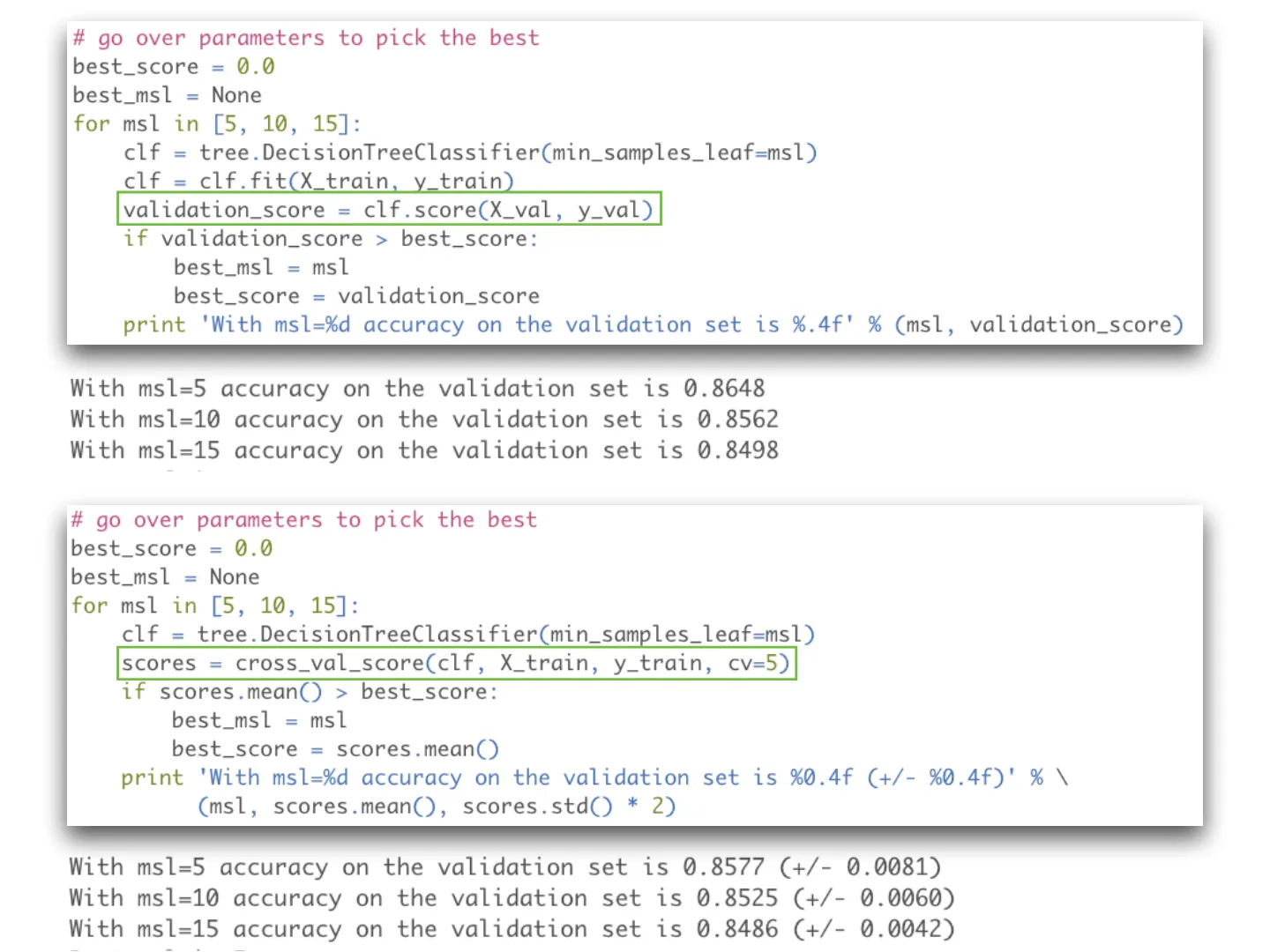
An introductory talk on the essential concepts of machine learning, given at the Mooncascade ML Camp 2016. It follows one use case, recognising handwritten digits, from start to finish: turning raw data into feature vectors, training a decision tree, measuring accuracy with a confusion matrix (and why accuracy misleads on an imbalanced dataset), overfitting and underfitting, splitting the data into training, validation and test sets, and cross-validation.
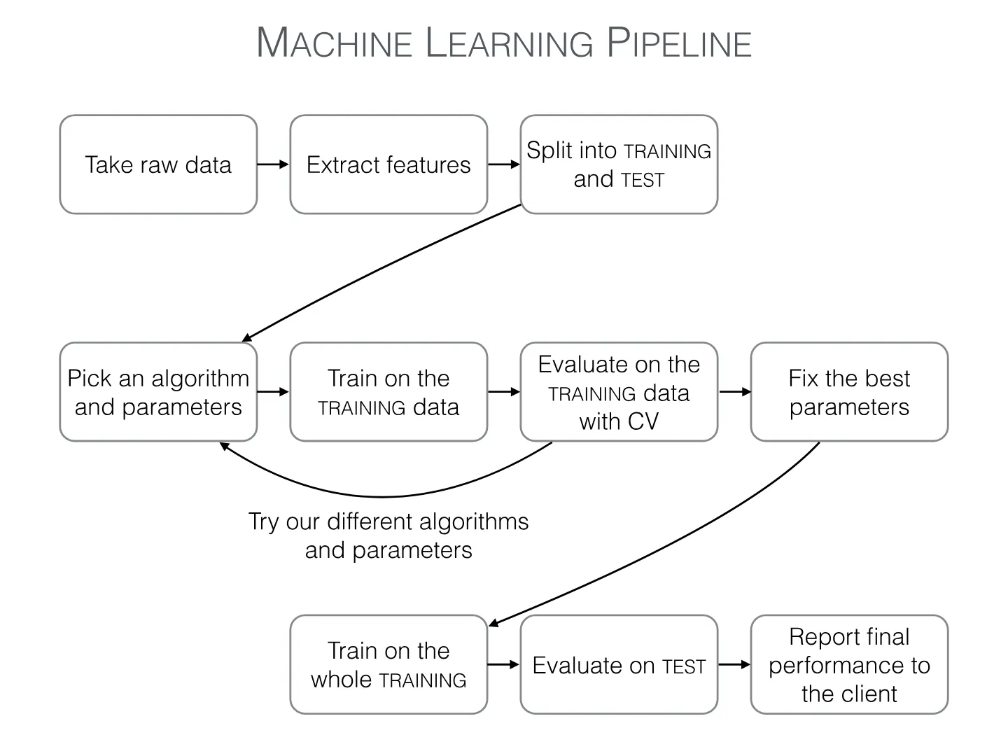
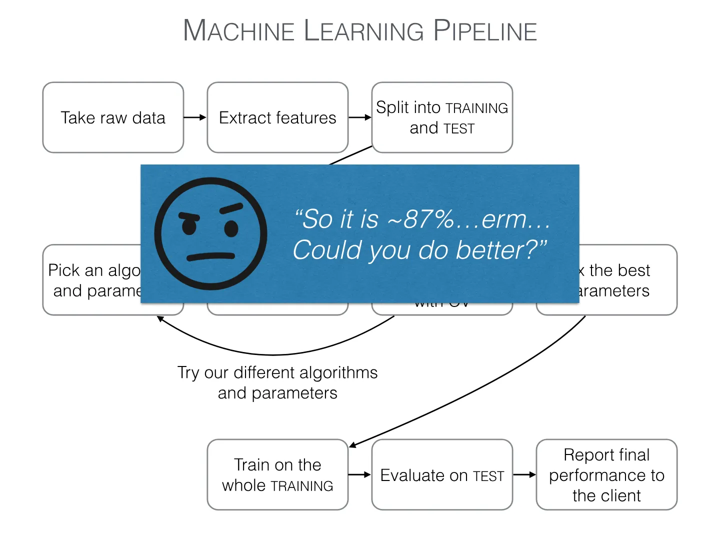
These steps come together as a machine learning pipeline, which is then improved by replacing the decision tree with a random forest. The talk closes with a look at how the same recipe applies to sound, text, images, video and database records, followed by a hands-on session with scikit-learn.

Download PDF